Let’s Revive an Old Idea
There are several ways to introduce the trigonometric functions: we can define them as ratios of sides in a right triangle, or in terms of the x- and y-coordinates of a point P on the unit circle, or as “wrapping functions” from the reals to some subset of the reals, or again as certain power series of the independent variable. Each approach has its merits, but clearly not all are equally suitable in the classroom. As I have mentioned in the Preface, the so-called “New Math” has imposed on trigonometry the language and formalities of abstract set theory—certainly not the best way to motivate the beginning student. I would like to suggest that we go back to an old idea: interpret the trigonometric functions as projections. To preempt criticism, let me say from the outset that nothing in this approach is new, but it reflects a shift in emphasis from the abstract to the practical. Let’s not forget that trigonometry is, first and foremost, a practical discipline, born out of and deeply rooted in applications.
In figure 100, let P(x, y) be a point on the unit circle, and let the angle between the positive x-axis and OP be θ (measured in degrees or radians). We define cos θ and sin θ as the projections of OP on the x- and y-axes, respectively. Since OP = 1, these projections are simply the x- and y-coordinates of the point P:
cos θ = OR = x, sin θ = PR = y.
The tangent function is defined as tan θ = y/x, but this too can be viewed as a projection: referring again to fig. 100, draw the vertical tangent line to the unit circle at the point S(1, 0), and call this line the t-axis. Extend OP until it meets the t-axis at Q. We have tan θ = y/x = PR/OR. But triangles OPR and OQS are similar, and therefore PR/OR = QS/OS. Recalling that OS = 1 and denoting the line segment QS by t, we have
tan θ = QS = t.
Thus tan θ is the projection of OP on the t-axis. The function cot θ can be similarly defined as the projection of OP on the horizontal tangent line to the circle at T(0, 1) (fig. 101); we have
cot θ = QT = c.
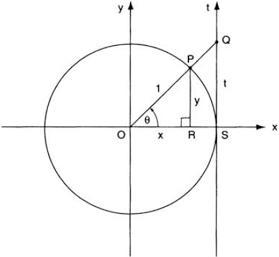
FIG. 100. The cosine, sine, and tangent functions as projections of the unit circle: OR = x = cos θ, RP = y = sin θ, SQ = t = tan θ.
So far the segments OR, PR, and QS were nondirected, but let us now think of them as directed line segments. This immediately leads us to conclude that tan θ is positive for 0° < θ < 90° (i.e., in quadrant I) and negative for 270° < θ < 360° (quadrant IV). If θ is in quadrant II, we project OP backward until it meets the t-axis at Q (fig. 102); since triangles OPR and OP′R′ are congruent, we have tan θ = PR/OR = P′R′/OR′ = SQ/1 = t, so that tan θ is now the negative line segment SQ. If θ is in quadrant III, projecting OP backward gives us again a positive value for SQ; we have here a geometric demonstration of the identity tan (θ + 180°) = tan θ.
As for sec θ and csc θ, they too can be interpreted (indeed defined) as projections: again let P be a point on the unit circle (fig. 103); draw the tangent line to the circle at P and extend it until it meets the x- and y-axes at M and N, respectively. We have ∠OPM = 90°, so that triangles OPR and OMP are similar; hence sec θ = 1/x = OP/OR = OM/OP = OM/1, so that the line segment OM represents the value of sec θ (again, it is a directed line segment, being negative when P is in quadrants II and III). Similarly, the line segment ON represents the value of csc θ. Moreover, since M and N always lie outside the circle, we see that the range of sec θ and csc θ is (−∞, −1] ∪ [1, ∞).
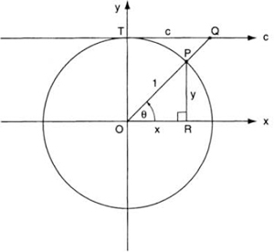
FIG. 101. The cotangent function as a projection: TQ = c = cot θ.
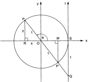
FIG. 102. The case when θ is in quadrant II.
Viewing all six trigonometric functions as projections allows us to see, quite literally, how these functions vary with θ: we only need to follow the various line segments as P moves around the circle. For example, to an observer watching from above, cos θ would appear as the to-and-fro motion of the “shadow” of P on the x-axis. This is even more dramatically illustrated in the case of tan θ: as θ increases, the shadow of P on the t-axis (point Q) rises slowly at first, than at an ever-increasing rate until it disappears at infinity as θ approaches 90°. Like the sweeping beam of a strobe light illuminating a dark wall, we have here a vivid graphic illustration of the peculiar behavior of tan θ near its asymptotes.1
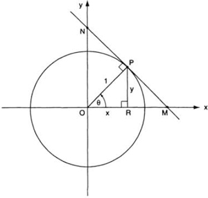
FIG. 103. The secant and cosecant functions as projections: OM = 1/x = sec θ, ON = 1/y = csc θ.
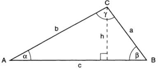
FIG. 104. The Law of Sines and the Law of Cosines as projections.
![]()
The concept of projection can be put to good use not only in defining the trigonometric functions. Consider any triangle ABC (fig. 104). Drop the perpendicular h from C to AB. The projections of the sides a and b on h—let’s call them the “vertical projections”—must of course be equal; hence
![]()
or a/sin α = b/sin β. Repeating this argument for sides b and c, we get b/sin β = c/sin γ; thus a/sin α = b/sin β = c/sin γ, which is the Law of Sines.
On the other hand, the projections of a and b on AB (the “horizontal projections”) must add up to the length of AB, that is, to c; we thus have
![]()
with similar equations for a and b (note that the formula is valid even if one angle, say α, is obtuse, in which case cos α will be negative). It would be entirely appropriate to call equation (2) the Law of Cosines (a name usually given to the more familiar formula c2 = a2 + b2 − 2ab cos γ)—all the more so because it involves two cosines, thus justifying the plural “s.” As an immediate consequence of equation (2) we have
![]()
with equality if, and only if, α = β = 0°. This is the famous triangle inequality.
Because it involves five variables—two angles and three sides—the usefulness of equation (2) for solving triangles is rather limited. We can, however, use equations (1) and (2) together to reduce the number of variables. Squaring equation (2), we have
c2 = a2 cos2 β + b2 cos2 α + 2ab cos α cos β
= a2(1 − sin2 β + b2(1 − sin2 α) + 2ab cos α cos β
= a2 + b2 − (a sin β)(a sin β) − (b sin α)(b sin α) + 2ab cos α cos β.
Using equation (1), we can write this as
= a2 + b2 − (a sin β)(b sin α) − (a sin β)(b sin α) + 2ab cos α cos β
= a2 + b2 + 2ab(cos α cos β − sin α sin β)
= a2 + b2 + 2ab cos (α + β).
But cos (α + β) = cos (180° − γ) = −cos γ; we thus get
![]()
which is the familiar form of the Law of Cosines. Thus the sine and the cosine laws simply express the fact that in a triangle, the perpendicular from any vertex to the opposite base is the vertical projection of either of the adjacent sides, and the base is the sum of their horizontal projections.
NOTE
1. Regrettably, many textbooks plot the graphs of tan θ and cot θ based on just a few scattered values of θ (in one case, as few as three!), arbitrarily chosen between −90° and 90°. Surely no real understanding of the peculiar behavior of these functions can be gained this way.