
OVERVIEW
1.1 INTRODUCTION
The performance of surface-sited radar against low-flying targets has been limited by land clutter since the earliest days of radar. Consider the beam of such a radar scanning over the surrounding terrain and illuminating it at grazing incidence. The amplitudes of the clutter returns received from all the spatially distributed resolution cells within the scan coverage on the ground vary randomly over extremely wide dynamic ranges, as the interrogating pulse encounters the complex variety of surface features and discrete reflecting objects comprising or associated with the terrain. The resultant clutter signal varies in a complex manner with time and space to interfere with and mask the much weaker target signal in the radar receiver. Early ground-based radars of necessity were restricted to operations at relatively long ranges beyond the clutter horizon where terrain was not directly illuminated. The development of Doppler signal processing techniques allowed radars to have capability within clutter regions against larger targets by exploiting the differences in frequency of the signal returned from the rapidly moving target compared to that from the relatively stationary clutter. However, because the clutter signal is often overwhelmingly stronger than the target signal and because of the lack of perfect waveform stability, modern pulsed radars often remain severely limited by land clutter residues against small targets even after clutter cancellation.
The need of designers and analysts to accurately predict clutter-limited radar system performance led to many attempts to measure and model land clutter over the decades following World War II [1–13]. The problem was highly challenging, not just because of the variability and wide dynamic range of the clutter at a given site, but also because the overall severity of the clutter and resulting system performance varied dramatically from site to site. Early clutter measurements, although numerous, tended to be low-budget piece-part efforts overly influenced by terrain specificity in each measurement scene. In aggregate these efforts led to inconsistent, contradictory, and incomplete results. Early clutter models tended to be overly general, modeling clutter simply as a constant reflectivity level, or on a spherical but featureless earth, or as a simple function of grazing angle. As a result, they did not incorporate features of terrain specificity that dominated clutter effects at real sites. Thus there was a logical disconnection between models (overly general) and measurements (overly specific), and clutter-limited radar performance remained unpredictable into the decade of the 1970s. By that time it had become widely acknowledged that “there was no generally accepted clutter model available for calculation,” and there was “no accepted approach by which a model could be built up” [8].
The middle and late 1970s also saw an emerging era of low-observable technology in aircraft design and consequent new demands on air defense capabilities in which liabilities imposed by the lack of predictability of clutter-limited surface radar performance were much heightened. As a result, a significant new activity was established at Lincoln Laboratory in 1978 to advance the scientific understandings of air defense. An important initial element of this activity was the requirement to develop an accurate full-scale clutter simulation capability that would breach the previous impasse. The goal was to make clutter modeling a proper engineering endeavor typified by quantitative comparison of theory with measurement, and so allow confident prediction of clutter-limited performance of ground-sited radar.
It was believed on the basis of the historical evidence that a successful approach would have to be strongly empirical. To this end, a major new program of land clutter measurements was initiated at Lincoln Laboratory [14–18]. To solve the land clutter modeling problem, it was understood that the new measurements program would have to substantially raise the ante in terms of level of effort and new approaches compared with those undertaken in the past. Underlying the key aspect of variability in the low-angle clutter phenomenon was the obvious fact that landscape itself was essentially infinitely variable—every clutter measurement scenario was different. Rather than seek the general in any individual measurement, underlying trends among aggregates of similar measurements would be sought.
In ensuing years, a large volume of coherent multifrequency land clutter measurement data was acquired (using dedicated new measurement instrumentation) from many sites widely distributed geographically over the North American continent [14]. A new site-specific approach was adopted in model development, based on the use of digitized terrain elevation data (DTED) to distinguish between visible and masked regions to the radar, which represented an important advance over earlier featureless or sandpaper-earth (i.e., statistically rough) constructs [15]. Extensive analysis of the new clutter measurements database led to a progression of increasingly accurate statistical clutter models for specifying the clutter in visible regions of clutter occurrence. A key requirement in the development of the statistical models was that only parametric trends directly observable in the measurement data would be employed; any postulated dependencies that could not be demonstrated to be statistically significant were discarded. As a result, a number of earlier insights into low-angle clutter phenomenology were often understood in a new light and employed in a different manner or at a different scale so as to reconcile with what was actually observed in the data. In addition, significant new advances in understanding low-angle clutter occurred that, when incorporated properly with the modified earlier insights, led to a unified statistical approach for modeling low-angle clutter in which all important trends observable in the data were reproducible.
An empirically-based statistical clutter modeling capability now exists at Lincoln Laboratory. Clutter-limited performance of surface-sited radar in benign or difficult environments is routinely and accurately predicted. Time histories of the signal-to-clutter ratios existing in particular radars as they work against particular targets at particular sites are computed and closely compared to measurements. Systems computations involving tens or hundreds of netted radars are performed in which the ground clutter1 at each site is predicted separately and specifically. Little incentive remains at Lincoln Laboratory to develop generic non-site-specific approaches to clutter modeling for the benefit of saving computer time, because the results of generic models lack specific realism and, as a result, are difficult to validate.
This book provides a thorough summary and review of the results obtained in the clutter measurements and modeling program at Lincoln Laboratory over a 20-year period. The book covers (1) prediction of clutter strength (Weibull statistical model2), (2) clutter spreading in Doppler (exponential model), and (3) given the strength and spreading of clutter, the extent to which various techniques of clutter cancellation (e.g., simple delay-line cancellation vs coherent signal processing) can reduce the effects of clutter on target detection performance.
1.2 HISTORICAL REVIEW
Although most surface-sited radars partially suppress land clutter interference from surrounding terrain to provide some capability in cluttered spatial regions, the design of clutter cancellers requires knowledge of the statistical properties of the clutter, and the clutter residues remaining after cancellation can still strongly limit radar performance (see Chapter 6, Sections 6.4.4 and 6.5). Because of this importance of land clutter to the operations of surface radar, there were very many early attempts [1–9] to measure and characterize the phenomenon and bring it into analytic predictability. A literature review of the subject of low-angle land clutter as the Lincoln Laboratory clutter measurement program commenced found over 100 different preceding measurement programs and over 300 different reports and journal articles on the subject. There exist many excellent sources of review [19–25] of these early efforts and preceding literature. These reviews without exception agree on the difficulty of generally characterizing low-angle land clutter.
The difficulty arises largely because of the complexity and variability of land-surface form and the elements of land cover that exist at a scale of radar wavelength (typically, from a few meters to a few centimeters or less) over the hundreds or thousands of square kilometers of composite terrain that are usually under radar coverage at a typical radar site. As a result, the earlier efforts [1–9] to understand low-angle land clutter revealed that it was a highly non-Gaussian (i.e., non-noise-like), multifaceted, relatively intractable, statistical random process of which the most salient attribute was variability. The variability existed at whatever level the phenomenon was observed—pulse-to-pulse, cell-to-cell, or site-to-site.
Other important attributes of the low-angle clutter phenomenon included: patchiness in spatial occurrence [3–5]; lack of homogeneity and domination by point-like or spatially discrete sources within spatial patches [6–8]; and extremely widely-skewed distributions of clutter amplitudes over spatial patches often covering six orders of magnitude or more [1, 2, 4, 9]. Early efforts to capture these attributes and dependencies in simple clutter models based only on range or illumination angle to the clutter cell were largely unsuccessful in being able to predict radar system performance. Figure 1.1 shows a measured plan-position-indicator (PPI) clutter map that illustrates to 24-km range at a western prairie site the spatial complexity and variability of low-angle land clutter. The fact that the clutter does not occur uniformly but is spatially patchy over the region of surveillance is evident in this measurement, as is the granularity or discrete-like nature of the clutter such that it often occurs in spatially isolated cells over regions where it does occur.

FIGURE 1.1 Measured X-band ground clutter map; Orion, Alberta. Maximum range = 24 km. Cells with discernible clutter are shown white. A large clutter patch (i.e., macroregion) to the SSW is also shown outlined in white.
Although the earlier efforts and preceding literature did not lead to a satisfactory clutter model, they did in total gradually develop a number of useful insights into the complexity of the land clutter phenomenon. Section 1.2 provides a summary of what these insights were, and the general approaches extant for attempting to bring the important observables of low-angle clutter under predictive constructs, as the Lincoln Laboratory program commenced.
1.2.1 CONSTANT σ°
Initially, land clutter was conceptualized (unlike Figure 1.1) as arising from a spatially homogeneous surface surrounding the radar site, of uniform roughness (like sandpaper) at a scale of radar wavelength to account for clutter backscatter. The backscatter reflectivity of this surface was characterized as being a surface-area density function, that is, by a clutter coefficient σ° defined [20] to be the radar cross section (RCS) of the clutter signal returned per unit terrain surface-area within the radar spatial resolution cell (see Section 2.3.1.1). This characterization implies a power-additive random process, in which each resolution cell contains many elemental clutter scatterers of random amplitude and uniformly distributed phase, such that the central limit theorem applies and the resultant clutter signal is Rayleigh-distributed in amplitude (like thermal noise).
As conceptualized in this simple manner, land clutter merely acts to uniformly raise the noise level in the receiver, the higher noise level being directly determined by σ°. A selected set of careful measurements of σ° compiled in tables or handbooks for various combinations of terrain type (forest, farmland, etc.) and radar parameter (frequency, polarization) would allow radar system engineers to straightforwardly calculate signal-to-clutter ratios and estimate target detection statistics and other performance measures on the basis of clutter statistics being like those of thermal noise, but stronger. Early radar system engineering textbooks promoted this view. However, this approach led to frustration in practice. Tabularization of σ° into generally accepted, universal values proved elusive. Every measurement scenario seemed overly specific. Resulting matrices of σ° numbers compiled from different investigators using different measurement instrumentation operating at different landscape scales (e.g., long-range scanning surveillance radar vs short-range small-spot-size experiments) and employing different data reduction procedures were erratic and incomplete, with little evidence of consistency, general trend, or connective tissue.
1.2.2 WIDE CLUTTER AMPLITUDE DISTRIBUTIONS
Clutter measurements that involved accumulating σ° returns by scanning over a spatially continuous neighborhood of generally similar terrain (i.e., clutter patch) found that the resulting clutter spatial amplitude distributions were of extreme, highly skewed shapes very much wider than Rayleigh [2, 4, 9]. Unlike the narrow fixed-shape Rayleigh distribution with its tight mean-to-median ratio of only 1.6 dB, the measured broad distributions were of highly variable shapes with mean-to-median ratios as high as 15 or even 30 dB.
Figure 1.2 shows five measured clutter histograms from typical clutter patches such as that shown in Figure 1.1, illustrating the wide variability in shape and broad spread that occurs in such data. Thus in the important aspect of its amplitude distribution, low-angle land clutter was decidedly non-noise-like. This fact was at best only awkwardly reconcilable with the constant-σ° clutter model. The accompanying shapes of clutter distributions as well as their mean σ° levels required specification against radar and environmental parameters, compounding the difficulties of compilation. As a result of both sea and land clutter measured distributions being wider than Rayleigh, an extensive literature came into being that addressed radar detection statistics in non-Rayleigh clutter backgrounds of wide spread typically characterizable as lognormal, Weibull, or K-distributed [26–31]. However, the need continued for a single-point constant-σ° clutter model to provide an average indication of signal-to-clutter ratio which left the user with the nebulous question of what single value of σ° (e.g., mean, median, mode, etc.) to use to best characterize the wide underlying distributions. Some investigators used the mean, others used the median, and it was not always clear what was being used since it did not make much difference under Rayleigh statistics and the question of underlying distribution was not always raised.

FIGURE 1.2 Histograms of measured clutter strength σ°F4 from five different clutter patches showing wide variability in shape and broad spread. σ° = clutter coefficient (see Section 2.3.1.1); F = pattern propagation factor (see Section 1.5.4). Black values are receiver noise.
1.2.3 SPATIAL INHOMOGENEITY/RESOLUTION DEPENDENCE
The definition of σ° as an area-density function implies spatial homogeneity of land clutter. The underlying necessary condition for the area-density concept to be valid is that the mean value of σ° be independent of the particular cell size or resolution utilized in a given clutter spatial field.3 As mentioned, it was additionally presumed that much the same invariant value of σ° (tight Rayleigh variations) would exist among the individual spatial samples of σ° independent of cell size. Early low-resolution radars showed land clutter generally surrounding the site and extending in range to the clutter horizon in an approximately area-extensive manner. Measurements at higher resolution with narrower beams and shorter pulses showed that clutter was not present everywhere as from a featureless sandpaper surface, but that resolved clutter typically occurred in patches or spatial regions of strong returns separated by regions of low returns near or at the radar noise floor [4]—see Figure 1.1. Thus, clutter was highly non-noise-like not only in its non-Rayleigh amplitude statistics, but also in its lack of spatial homogeneity. Highresolution radars took advantage of the spatial non-homogeneity of clutter by providing some operational capability known as interclutter visibility in relatively clear regions between clutter patches [23].
Within clutter patches, clutter is not uniformly distributed. The individual spatial samples of σ°, as opposed to their mean, depend strongly upon resolution cell size. Thus the shapes of the broad amplitude distributions of σ° are highly dependent on resolution—increasing resolution results in less averaging within cells, more cell-to-cell variability, and increasing spread in values of σ°. In contrast, the fixed shape of a Rayleigh distribution describing simple homogeneous clutter is invariant with resolution. Significant early work was conducted into establishing necessary and sufficient conditions (e.g., number of scatterers and their relative amplitudes) in order for Rayleigh/Ricean statistics to prevail in temporal variations from individual cells, but the associated idea of how cell size affects shapes of spatial amplitude distributions from many individual cells was less a subject of investigation.
One early study got so far as to document an observed trend of increasing spread in clutter spatial amplitude distributions with increasing radar resolution [8], but this fundamentally important observation into the nature of low-angle clutter4 was not generally followed up on or worked into empirical clutter models. Figure 1.3 shows how the Weibull shape parameter aw (see Section 2.4.1.1), which controls the extent of spread in histograms such as those of Figure 1.2, varies strongly with radar spatial resolution in low-relief farmland viewed at low depression angle. These and many other such results for various terrain types and viewing angles are presented and explained in Chapter 5.

FIGURE 1.3 Weibull shape parameter aw vs resolution cell area A for low-relief farmland viewed at low depression angle. Plot symbols are defined in Chapter 5. These data show a rapid decrease in the spread of measured clutter spatial amplitude statistics with increasing cell size (each plot symbol is a median over many patch measurements). aw = 1 represents a tight Rayleigh (voltage) distribution with little spread (mean/median ratio = 1.6 dB). aw = 5 represents a broadly spread Weibull distribution (mean/median ratio = 28.8 dB).
These two key attributes of low-angle clutter—patchiness and lack of uniformity in spatial extent (Figure 1.1), and extreme resolution-dependent cell-to-cell variability in clutter amplitudes within spatial patches of occurrence (Figures 1.2 and 1.3)—do not constitute extraneous complexity to be avoided in formulating simple clutter models aimed at generality, but in fact are the important aspects of the phenomenon that determine system performance and that therefore must be captured in a realistic clutter model.
1.2.4 DISCRETE CLUTTER SOURCES
The increasing awareness of the capability of higher resolution radars to resolve spatial feature and structure in ground clutter and see between clutter patches led to investigations using high resolution radars to determine the statistics of resolved patch size and patch separation as a function of thresholded strength of the received clutter signal. It was found that the spatial extents of clutter patches diminished with increasing signal-strength threshold such that in the limit the dominant land clutter signals came from spatially isolated or discrete point sources on the landscape (e.g., individual trees or localized stands of trees; individual or clustered groups of buildings or other man-made structures; utility poles and towers; local heights of land, hilltops, hummocks, river bluffs, and rock faces) [6, 7]. This discrete or granular nature of the strongest clutter sources in low-angle clutter became relatively widely recognized—this granularity is quite evident in Figure 1.1. It became typical for clutter models to consist of two components: a spatially-extensive background component modeled in terms of an area-density clutter coefficient σ°, and a discrete component modeled in terms of radar cross section (RCS) as being the appropriate measure for a point source of clutter isolated in its resolution cell and for which the strength of the RCS return is independent of the size of the cell encompassing it. The RCS levels of the discretes were specified by spatial incidence or density (so many per square km), with the incidence diminishing as the specified level of discrete RCS increased. Note that in such a representation for the discrete clutter component, although the strength of the RCS return from a single discrete source is independent of the spatial resolution of the observing radar, the probability of a cell capturing zero vs one vs more than one discrete does depend on resolution (i.e., discrete clutter is also affected by cell size). It was usual in such two-component clutter models for the extended background σ° component to be developed more elaborately than the discrete RCS component, the latter usually being added in as an adjunct overlay to what was regarded as the main area-extensive phenomenon.
Although the two-component clutter model seemed conceptually simple and satisfactory as an idealized concept to deal with first-level observations, attempting to sort out measured data following this approach was not so simple. The wide measured spatial amplitude distributions of clutter were continuous in clutter strength over many (typically, as many as six or eight) orders of magnitude and did not separate nicely into what could be recognized as a high-end cluster of strong discretes and a weaker bell-curve background. That is, in measured clutter data, there is no way of telling whether any given return is from a spatially discrete or distributed clutter source [25]. Additional complication arises due to radar spatial resolution diminishing linearly with range (i.e., cross-range resolution is determined by azimuth beamwidth) so that discretes of a given spatial density might be isolated at short range but not at longer ranges. The reality is that, at lower signal-strength thresholds, spatial cells capture more than one discrete and cell area affects returned clutter strength. This difficulty in the two-component model of how to transition in measured data and hence in modeling specification between extended σ° and discrete RCS has been discussed very little in the literature. These matters are discussed more extensively in Chapter 4, Section 4.5.
1.2.5 ILLUMINATION ANGLE
To many investigators, a land clutter model is basically just a characteristic of σ° vs illumination angle in the vertical plane of incidence. The empirical relationship σ° = γ sin ψ where ψ is grazing angle (i.e., the angle between the terrain surface and the radar line-of-sight; see Figure 2.15 in Chapter 2) and γ is a constant dependent on terrain type and radar frequency has come to be accepted as generally representative over a wide range of higher, airborne-like angles [24]. However, at the low angles of ground-based radar, typically with ψ < 1° or 2°, it was not clear how to proceed. One relatively widely-held school of thought5 was that at such low angles in typically-occurring low-relief terrain, grazing angle was a rather nebulous concept, neither readily definable [e.g., at what scale should such a definition be attempted, that of radar wavelength (cm) or that of landform variation (km)?] nor necessarily very directly related to the clutter strengths arising from discontinuous or discrete sources of vertical discontinuity dominating the low-angle backscatter and principally associated with land cover. From this point-of-view, the radar wave was more like a horizontally-propagating surface wave than one impinging at an angle from above, and it made more sense to separate the clutter by gross terrain type (mountains vs plains, forest vs farmland) than by fine distinctions in what were all very oblique angles of incidence.
Another widely held school-of-thought was to extend the constant-γ model to the low-angle regime by adding a low-angle correction term to prevent σ° from becoming vanishingly small at grazing incidence (as ψ → 0°). Little appropriate measurement data (for example, from in situ surveillance radars) was available upon which to base such a corrective term. Moreover, the idea of a corrective term tends to oversimplify the low-angle regime. At higher angles, the assumption behind a constant-γ model is of Rayleigh statistics; at low angles, it was known that the shapes of clutter amplitude distributions were broader and modelable as Weibull or lognormal, but following through with information specifying shape parameters continuously with angle for corrected constant-γ models at low angles was generally not attempted.
The gradually increasing availability of digitized terrain elevation data (DTED) in the 1970s and 1980s, typically at about 100 m horizontal sampling interval and 1 m quantization in elevation, quickly led to its use by the low-angle clutter modeling community. The hope was that the DTED would carry the burden of terrain representation by allowing the earth’s surface to be modeled as a grid of small interconnected triangular DTED planes or facets joining the points of terrain elevation. Then clutter modeling could proceed relatively straightforwardly in the low-angle regime, as a function of grazing angle (e.g., constant-γ or extended constant-γ) on inclined DTED facets. This approach to modeling low-angle clutter won a wide following and continues to receive much attention. Note that it is usually advocated as a seemingly sensible but unproven postulate, and not on the basis of successful reduction of actual measurement data via grazing angle on DTED facets. As applied on a cell-by-cell (or facet-by-facet) basis, such a model is usually thought of as returning deterministic samples of σ°, thus avoiding the difficult problem of specifying statistical clutter spreads at low angles (although such a model can return random draws from statistical distributions if the distributions are specified). Indeed, when applied deterministically, the cell-to-cell scintillations in the simulated clutter signal caused by variations in DTED facet inclinations appear to mimic scintillation in measured clutter signals. However, this simple deterministic approach to modeling generally does not result in predicted low-angle clutter amplitude distributions matching measurement data. Predicted signal-to-clutter ratios and track errors recorded in radar tracking of low-altitude targets across particular clutter spatial fields using such a model show little correlation with measured data.
The root cause of this failure is that the bare-earth DTED-facet representation of terrain does not carry sufficient information to alone account for radar backscatter; it lacks precision and accuracy to define terrain slope at a scale of radar wavelength and provides no information on the discrete elements of land cover which dominate and cause scintillation in the measurement data. This is illustrated by the results of Figure 1.4. At the top, Figure 1.4(a) shows X-band measurements of clutter strength vs grazing angle in two short-range canonical situations where the clutter-producing surface was very level—on a frozen snow-covered lake and on an artificially level, mown-grass, ground-reflecting antenna range. In such situations, the computation of grazing angle is straightforward—it is simply equal to the depression angle below the horizontal at which the clutter cell is observed at the radar antenna. In these two canonical or laboratory-like measurement situations, a strong dependence of increasing clutter strength with increasing grazing angle is indicated.

FIGURE 1.4 Measurements of clutter strength σ°F4 vs grazing angle. (a) Canonically level, discrete-free surfaces; (b) undulating open prairie landscape.
Such results illustrate the thinking that lies behind the desire of many investigators to want to establish a grazing-angle dependent clutter model. However, as shown in Figure 1.4(b), when grazing angle is computed to DTED facets used to model real terrain surfaces, little correlation between clutter strength and grazing angle is seen in the results. Specifically, Figure 1.4(b) shows a scatter plot in which measured X-band clutter strength in each cell at the undulating western prairie site of Beiseker, Alberta is paired with an estimate of grazing angle to the cell derived from a DTED model of the terrain at the site. As mentioned, the reasons that little or no correlation is seen in the results have to do with lack of accuracy in the DTED and in the fact that the bare-earth DTED representation of the terrain surface contains no information on the spatially discrete land cover elements that usually dominate low-angle clutter. Results such as those shown in Figure 1.4(b) are discussed at greater length in Chapter 2 (see Section 2.3.5). Such results illustrate why attempting deterministic prediction of low-angle clutter strength via grazing angle to DTED facets has been an oversimplified micro-approach that fails.
1.2.6 RANGE DEPENDENCE
Return now to the first school of thought mentioned in the preceding discussion concerning illumination angle, namely, that at grazing incidence in low-relief terrain, terrain slope and grazing angle are neither very definable nor of basic consequence in low angle clutter. Within this school of thought, the central observable fact concerning clutter in a ground-based radar is its obvious dissipation with increasing range. Thus some early clutter models for surface-sited radars were formulated from this point of view. Rather than model the clutter at microscale, such models treated the earth as a large featureless sphere, uniformly microrough to provide backscattering, but without specific large-scale terrain feature. Such an earth does not provide spatial patchiness; rather it is uniformly illuminated everywhere to the horizon, and clutter strength is diminished with increasing range via propagation losses over the spherical earth. This appears to be a simple general macroscale approach for providing a range-dependent clutter model for surface-sited radar.
However, like the microscale grazing angle model, the macroscale range-dependent model does not conform to the measurement data. These data show that what actually diminishes with increasing range at real sites is the occurrence of the clutter—with increasing range, visible clutter-producing terrain regions become smaller, fewer, and farther between, until, beyond some maximum range, no more terrain is visible (see Chapter 4, Figure 4.10). Further, the measurement data show that clutter strength does not generally diminish with increasing range, either within visible patches or from patch to patch. To illustrate this, Figure 1.5 shows mean clutter strength vs range in a 20° azimuth sector at Katahdin Hill, Massachusetts, looking out 30 km over hilly forested terrain. The data in this figure scintillate from gate to gate and occasionally drop to the noise floor where visibility to terrain is lost, but the average level stays at ∼ −30 dB over the full extent in range with no significant general trend exhibited of, for example, decreasing clutter strength with increasing range. Many similar results from Katahdin Hill and other sites are discussed in detail in what follows (see Chapter 2, Section 2.3 and Chapter 4, Appendix 4.A).

FIGURE 1.5 Mean clutter strength σ°F4 vs range at Katahdin Hill. X-band data, averaged range gate by range gate within a 20°-azimuth sector, 80 samples per gate. Range gate sampling interval = 148.4 m. Such results indicate little general trend of clutter strength with range.
Another way of examining the measurement data for range dependence of clutter strength is in PPI clutter maps such as is shown in Figure 1.1. If a gradually increasing threshold on clutter strength is applied to a measured long-range PPI clutter map, the clutter does not disappear at long ranges first, but tends to uniformly dissipate within patches of occurrence over much of the PPI independent of range (see Chapter 4, Figure 4.19). Thus patchiness is necessary in a clutter model, not only to realistically represent the spatial nature of the clutter in local areas, but also to provide the important global feature of diminishing clutter occurrence (not strength) with increasing range.
1.2.7 STATUS
The preceding discussions give some sense as to the state of understanding of low-angle land clutter and different points of view regarding its modeling when the Lincoln Laboratory clutter program commenced. As has been indicated, various elements of this complex phenomenon were individually understood to greater or lesser degrees, but a useful overall prediction capability was not available. Next, Section 1.3 briefly describes the Lincoln Laboratory measurement equipment for obtaining an extensive new land clutter database of clutter for the development of new empirical clutter models. Then Section 1.4 takes up again the various facets of the clutter phenomenon introduced in the foregoing and shows how the successful predictive approaches developed in this book build on the thinking that went before but extend it in improved ways of analyzing the data and formulating the models.
1.3 CLUTTER MEASUREMENTS AT LINCOLN LABORATORY
The Lincoln Laboratory program of radar ground clutter measurements went forward in two main phases, Phase Zero [18], a pilot phase that was noncoherent and at X-band only, followed by Phase One [14], the full-scale coherent program at five frequencies, VHF, UHF, L-, S-, and X-bands. Photographs of the Phase Zero and Phase One measurement instruments are shown in Figures 1.6 and 1.7, respectively. The basis of the Phase Zero radar was a commercial marine navigation radar, in the receiver of which was installed a precision intermediate frequency (IF) attenuator to measure clutter strength. Phase Zero measurements were conducted at 106 different sites. The Phase One five-frequency radar was a one-of-a-kind special-purpose instrumentation radar specifically designed to measure ground clutter. It was computer-controlled with high data rate recording capability. It utilized a linear receiver with 13-bit analog-to-digital (A/D) converters in in-phase (I) and quadrature (Q) channels, and maintained coherence and stability sufficient for 60-dB clutter attenuation in postprocessing. Phase One five-frequency measurements were conducted at 42 different sites.


Important system parameters associated with the Phase Zero and Phase One radars are shown in Table 1.1. Both instruments were self-contained and mobile on truck platforms. Antennas were mounted on erectable towers and had relatively wide elevation beams that were fixed horizontally at 0° depression angle. That is, no control was provided on the position of the elevation beam. For most sites and landscapes, the terrain at all ranges from one to many kilometers was usually illuminated within the 3-dB points of the fixed elevation beamwidth. At each site, terrain backscatter was measured by steering the azimuth beam through 360° and selecting a maximum range setting such that all discernible clutter within the field of view, typically from 1 km to about 25 or 50 km in range, was recorded. The Phase Zero and Phase One radars had uncoded, pulsed waveforms.
TABLE 1.1
Clutter Measurement Parameters
| Phase Zero | Phase One | |
| Frequency | ||
| Band | X-Band | VHF UHF L-Band S-Band X-Band |
| MHz | 9375 | 165 435 1230 3240 9200 |
| Polarization | HH | VV or HH |
| Resolution | ||
| Range | 9, 75, 150 m | 15, 36, 150 m |
| Azimuth | 0.9° | 13° 5° 3° 1° 1° |
| Peak Power | 50 kW | 10 kW (50 kW at X-Band) |
| 10 km Sensitivity | σ°F4 = −45 dB | σ°F4 = −60 dB |
| Antenna Control | Continuous Azimuth Scan | Step or Scan through Azimuth Sector (<185°) |
| Tower Height | 50′ | 60′ or 100′ |
| Data | ||
| Volume | 2 Tapes/Site (800 bpi) | ≈ 25 Tapes/Site (6250 bpi) |
| Acquisition Time | 1/2 Day/Site | 2 Weeks/Site |
The Phase Zero and Phase One clutter measurement radars were internally calibrated for every clutter measurement. The Phase One instrument was externally calibrated at many sites, using standard gain antennas and corner reflectors mounted on portable towers. The Phase Zero instrument utilized balloon-borne spheres to provide several external calibrations. More detailed information describing the Phase Zero and Phase One clutter measurement radars is provided in Chapters 2 and 3, respectively.
Several years after the Phase One measurement program was completed, the L-band component of the Phase One radar was upgraded to provide an improved LCE (L-band Clutter Experiment) instrument for the measurement of low-Doppler windblown clutter spectra to low levels of clutter spectral power. The LCE radar is described in Chapter 6.
Figure 1.8 shows results of five-frequency measurements of ground clutter conducted by the Phase One instrument at 35 general rural sites. Each plotted point indicates the mean value of clutter strength σ°F4—F is the pattern propagation factor (see Section 1.5.4)—obtained from a particular clutter patch for given settings of radar frequency, polarization, and range resolution, one clutter patch per site from each of the 35 sites (Figure 1.1 shows the outline of a typical clutter patch). These results illustrate the variability in mean strength from measured clutter histograms (e.g., see the vertical dashed lines in Figure 1.2); the cell-to-cell variability within the clutter patches is usually much greater (indicated by the overall extent in σ°F4 of the histograms in Figure 1.2). Such variability in mean clutter strength as is indicated in Figure 1.8 occurs both due to variations in the intrinsic clutter coefficient σ° as well as variations in the propagation factor F (e.g., as discussed in Section 3.3.2). The five-frequency results of Figure 1.8 show broad site-to-site variability and increasing variability with decreasing radar frequency (i.e., 20 dB of variability at X-band increasing to 65 dB of variability at VHF); but otherwise indicate little general trend of mean clutter strength with radar frequency when averaged over all rural terrain types. In contrast and as will be demonstrated, significant trends of mean clutter strength with frequency do occur in specific rural terrain types (e.g., farmland vs forest). The results of Figure 1.8 are discussed in much greater detail in Chapter 3 (see Section 3.5.1).
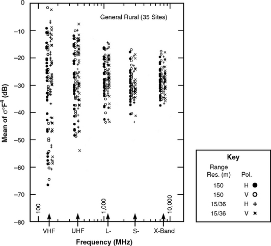
FIGURE 1.8 Mean clutter strength vs radar frequency in general rural terrain, as measured at 35 sites. These data show broad site-to-site variability, and increasing variability with decreasing frequency; but otherwise indicate little overall (e.g., medianized) trend of mean clutter strength with frequency.
1.4 CLUTTER PREDICTION AT LINCOLN LABORATORY
Section 1.4 describes the basic tenets underpinning ground clutter modeling efforts at Lincoln Laboratory and upon which the success of the models fundamentally depends. These tenets are further developed in subsequent sections of this book. Much of the discussion follows from the preceding historical review (Section 1.2) of important ideas that had emerged earlier concerning low-angle ground clutter and previous approaches to its modeling.
1.4.1 EMPIRICAL APPROACH
The approach to solving the problem of bringing order and predictability to low-angle clutter, as carried forward in this book, is based on trend analysis in measurement data. Averaging over large amounts of high-quality, internally self-consistent measurement data allows fundamental underlying trends to emerge which are often obscured by specific effects in individual measurements. No attempts are made to hypothesize and validate theoretical solutions, and any notional dependencies that cannot be demonstrated in the data are also not utilized. Empirical predictive constructs for low-angle clutter in surface radar are developed based on replicating all important general trends observed in the measurement data.
1.4.2 DETERMINISTIC PATCHINESS
As stated previously, the most salient characteristic of ground clutter in a surface radar is variability. One important way that this variability manifests itself is patchiness in spatial occurrence (see Figure 1.1). Clutter does not exist everywhere, and its on-again, off-again behavior is what fundamentally determines system performance at any given site. The main approach of this book presumes the use of DTED to deterministically approximate the site-specific spatial patterns of terrain visibility and hence clutter occurrence at each site of interest. Following this approach, answers about the degree to which clutter limits system performance are obtainable one site at a time. Clutter varies dramatically from site to site, and the extent to which clutter limits radar performance only has deterministic meaning on a site-specific basis. Some effort (coordinated with studies at Lincoln Laboratory) has been made elsewhere [32] to include mathematically-derived stochastic patchiness within a general non-site-specific clutter modeling framework, but in such efforts the statistics of patchiness, dependent upon terrain type, are themselves obtained from processing in DTED for the terrain type of interest. A site-specific deterministically-patchy model allows quantitative comparison between prediction and measurement of given clutter patches at given sites; more general stochastically-patchy or non-patchy models cannot be validated in this direct manner.
1.4.3 STATISTICAL CLUTTER
Although the visible regions of occurrences of ground clutter (i.e., the macroscale clutter spatial occupancy map—see Figure 1.1) are predicted deterministically using DTED, the clutter amplitudes that occur distributed over such regions are a statistical phenomenon. The information content in DTED is suitable for defining kilometer-sized macroregions of terrain visibility, but this information content—in currently available or any foreseeable database of digitized terrain elevations and/or terrain descriptive information—is insufficient to deterministically predict clutter amplitudes in individual spatial cells. Thus this book characterizes land clutter strength (as opposed to its spatial occupancy map) as a statistical random process and determines predictive parametric trends in the parameters characterizing the statistical clutter amplitude distributions.
1.4.4 ONE-COMPONENT σ° MODEL
The difficulty in two-component clutter models6 of how to transition in measured data and modeling specification between extended σ° and discrete RCS was previously brought into consideration in Section 1.2.4. Consider again the key role that spatial resolution plays in low-angle ground clutter (see Section 1.2.3). The shapes of clutter spatial amplitude distributions are highly dependent on resolution over their whole extents (not just their strong-side tails). This results from the fact that at grazing incidence much of the discernible clutter (not just the strongest returns) is discrete-like. This key fact has been relatively unrecognized in the clutter literature, although occasional past remarks may be found that begin to approach the idea. For example, Krason and Randig [3] based the interpretation of their measurements of forest clutter on what appeared to them to be a fundamental “transition from diffuse scattering at large angles to specular scattering at the very shallow angles.” Recall that surface clutter as originally conceptualized—wherein all cells, whether large or small, contain large numbers of small scatterers—provides amplitude distributions with unvarying tight Rayleigh shapes and no dependence of shape on resolution. In contrast, what the radar is actually collecting at low angles is a broad continuum of spiky returns from discretes over a wide range of amplitudes, such that there are usually a number of discretes in each cell. This number is small enough that changing cell size strongly affects the statistics of the results.
Recognition of this fact allows the complete spatial field of low-angle land clutter from weakest to strongest cells to be understood and predicted in a unified manner using an area-extensive σ° formulation. The approach properly deals with cells containing a number of relatively weak, randomly-phased discretes as a power-additive density function in the statistical aggregate of many such cells. However, the approach also properly treats occasional cells containing strong isolated discretes, despite the fact that representing isolated discretes with a density function may at first seem inappropriate. For such a cell, a high-resolution radar will contribute a strong σ° into a wide amplitude distribution, and a low-resolution radar will contribute a weaker σ° into a narrower amplitude distribution. Prediction of clutter RCS from these distributions will result in the same RCS for the large discrete in both cells (large σ° times small cell area equals smaller σ° times larger cell area).
Thus a statistical σ° model implementing the fundamental property of spread in amplitude distribution vs resolution can capture and recreate the observed spatial granularity and point-like nature of clutter fields at low angles of observation, without recourse to an additional RCS component that is difficult to implement realistically. The reasoning behind why the density function σ° is the proper way to model clutter even when dominated by discrete sources is considerably expanded upon in Chapter 4, Section 4.5. The clutter modeling statistics provided in this book follow this approach (but see Appendix 4.D).
1.4.5 DEPRESSION ANGLE
Return now to the preceding discussion (Section 1.2.5) of historical perceptions on whether illumination angle might be important in affecting low-angle clutter strength, and if so, how to implement it in a model. Another position on how to use illumination angle to help characterize low-angle clutter, intermediate between that of not using angle at all (following the first approach described in Section 1.2.5) and that based on fine-scale specification of local terrain slopes in DTED (following the subsequent approach described in Section 1.2.5), exists and was utilized in the early literature by Linell [1] to successfully reduce measurement data from a ground-sited radar working over ranges up to 12 km.7 Although terrain slopes may not be very definable or directly relatable to clutter strengths at grazing incidence (as under the first approach described in Section 1.2.5), this intermediate approach brings a more macroscopic measure of angle to bear on the problem, namely the depression angle at which larger patches of relatively uniform terrain are viewed below the local horizontal at the radar antenna. The use of DTED to define depression angle as a macroparameter in this manner is appropriate to the information content and accuracy of the DTED, in contrast to the use of DTED to define grazing angle as a microparameter associated with individual cells. That is, depression angle depends only on terrain elevations and not their rates of change and hence is a slowly varying quantity over clutter patches; whereas grazing angle depends also on rates of change of elevation (i.e., the derivative) and hence is a rapidly varying quantity much more susceptible to inaccuracies and error tolerances in DTED. Linell’s results [1] showed that levels and shapes of clutter amplitude distributions measured from such macropatches were extremely sensitive to the differences in depression angle (e.g., 0.7°, 1.25°, 5°) at which they were obtained. These data became widely referenced [21, 24, 26], but did not directly lead to clutter models. An important distinction is that such data did not directly provide a simple continuous angle characteristic (like constant-γ), but instead showed how complete clutter amplitude distributions vary in steps or intervals of depression angle regime.
Similar effects with depression angle, as first seen much earlier by Linell, both on the mean levels and shapes of clutter amplitude distributions over large spatial macroregions of low-angle clutter occurrence, constitute a highly pervasive and important parametric influence observed throughout the Phase Zero and Phase One measurements. Figure 1.9 shows these strong effects of depression angle on levels and shapes of clutter amplitude distributions. The curves of Figure 1.9 are plotted from the Phase Zero X-band data in Table 2.4 of Chapter 2; they were first presented in this manner by Skolnik [19]. It is evident in these results that mean and median clutter strengths rise rapidly with increasing depression angle, and that spreads in clutter amplitude distributions as given by either the mean/median ratio (as shown in the lower part of Figure 1.9) or by the Weibull shape parameter aw rapidly decrease with increasing angle (the upper part of Figure 1.9 plots the inverse of aw against depression angle). The results shown in Figure 1.9 are described in greater detail in Chapter 2.

FIGURE 1.9 General variation of ground clutter strength (mean and median) and spread (aw) in measured ground clutter spatial amplitude statistics vs depression angle, for rural terrain of low and high relief. Clutter strengths increase and spreads decrease with increasing depression angle. X-band data, plotted from Table 2.4 in Chapter 2. (After Skolnik [19]; by permission, © 2001 The McGraw-Hill Companies, Inc.)
Although Linell’s results reporting the sensitivity of shape parameter to angle were relatively widely referenced, the corresponding similar sensitivity of shape parameter to radar spatial resolution was less widely recognized, as of course were the consequent interdependent effects of angle and resolution together on shape. These important interdependent effects of both depression angle (Figure 1.9) and radar resolution (Figure 1.3) on the shapes of low-angle clutter amplitude distributions are key elements in the clutter modeling information provided in this book.
1.4.6 DECOUPLING OF RADAR FREQUENCY AND RESOLUTION
Statistical low-angle clutter amplitude distributions are fundamentally characterized by a mean absolute level, and by the shape or degree of spread (broad or narrow) about the mean level. Results in this book show that the mean level of the distribution depends strongly on radar frequency, depending on terrain type (see Figure 3.38);8 and that the shape of the distribution depends strongly on radar spatial resolution (as has been discussed, see Figure 1.3). In addition, both the mean level and the shape depend upon depression angle (see Figure 1.9). However, analyses of the clutter measurement data have uncovered an important further fact, fundamental to the development of the modeling information in this book. This further fact is the decoupling of the effects of radar frequency and resolution on the clutter amplitude distributions. Thus, although radar frequency affects mean level, it does not significantly affect shape; and although radar resolution affects shape, it does not affect mean level. The mean level is the only statistical attribute of the distribution unaffected by resolution; for example, the median and other percentile levels are strongly affected by resolution. This decoupling of effects of radar frequency and resolution on clutter amplitude distributions greatly decreases the parametric dimensionality of the consequent clutter modeling construct, such that this construct constitutes a proper empirical model incorporating trends over many measurements, and does not simply degenerate to a table look-up procedure of specific measurements.
1.4.7 RADAR NOISE CORRUPTION
At the very low angles at which surface radar illuminates the surrounding terrain, typically < 1° or 2°, even within spatial macroregions (i.e., clutter patches comprising many resolution cells) that are under general illumination and not deep in shadow, there usually occurs a subset of randomly occurring radar return samples from low-lying or shadowed terrain cells interspersed within the patch that are at the noise level of the radar (see Figure 1.2; samples at radar noise level shown black). This phenomenon is henceforth referred to as the occurrence of microshadow within macropatches of clutter. Microshadow is inescapable in low-angle clutter statistics. The correct way of dealing with microshadow is as follows: once the boundaries of a spatial clutter patch are defined (for example, by terrain visibility in DTED), all of the samples returned from within the patch boundaries must be included in the clutter statistics, including those at radar noise level. Frequently, in the clutter literature, only the shadowless or noise-free set of samples above radar noise level (shown white in Figure 1.2) is retained to characterize the clutter in the region. Shadowless statistics are dependent on the sensitivity of the measurement radar; that is, radars of differing sensitivity obtain different numbers of noise samples and hence obtain different measures of shadowless clutter strength. The key requirement for determining correct absolute measures of clutter strength over a given spatial patch of clutter (as opposed to relative, sensitivity-dependent measures) is to include all samples from the patch in the computation, including those at radar noise level. Clutter amplitude distributions from spatial patches inclusive of all the returns from the patch (including those at radar noise level) will henceforth be referred to as all-sample distributions.
The necessary existence of noise-level samples in all-sample clutter amplitude distributions is a source of corruption in clutter computation. This corruption is dealt with as follows. All statistical quantities including moments and percentile levels are computed and shown two ways: 1) as an upper bound in which samples at noise level keep their noise power values (for noise samples, the actual clutter power ≤ noise power); and 2) as a lower bound in which the samples at noise level are assigned zero or a very low value of power (for noise samples, the actual clutter power ≥ zero). The correct value of the statistical quantity, that is, the value that would be measured by a theoretically infinitely sensitive radar for which the upper and lower bounds would coalesce, must lie between the upper bound and lower bound values. Even when the amount of noise corruption is severe, upper and lower bounds to statistical moments are usually close to one another because these calculations are dominated by the strong returns from the discrete clutter sources within the patch. In contrast, moments and percentile levels in the less correct, noise-free or shadowless distributions can be significantly higher than upper and lower bounds to these quantities in the corresponding, more correct noise-corrupted all-sample distributions. Separation of upper and lower bound values by large amounts in all-sample distributions indicates a measurement too corrupted by noise to provide useful information.
The modeling information provided in this book is based on noise-corrupted all-sample clutter amplitude distributions from measured clutter patches with tight upper and lower bounds. As a consequence, the Weibull distributions specified herein for predicting clutter amplitude distributions cover all the cells and samples in a given patch including those at noise level for a radar of given sensitivity. That is, the Weibull distributions specify the clutter as appropriate for an infinitely sensitive radar; a subsequent system-dependent calculation is required to determine the subset of weak Weibull clutter values that are predicted below system noise level for the particular radar and clutter patch being modeled. In this manner, the modeling approach of this book correctly provides absolute measures of clutter strength not dependent on Phase Zero or Phase One radar measurement sensitivities and correctly includes microshadow in predicted low-angle clutter amplitude distributions for a modeled radar depending on its specific sensitivity, which can be different from that of the Phase Zero and Phase One clutter measurement radars.
1.5 SCOPE OF BOOK
The subject matter of this book is the phenomenology of low-angle land clutter in surface-sited radar. Trend analyses are conducted of the measured ground clutter data, and empirical modeling of clutter based on the trends revealed is performed. Section 1.5 describes the overall scope of the material to follow, including the ranges in important radar and environmental parameters over which clutter modeling information is subsequently presented and to which this information is limited.
1.5.1 OVERVIEW
A surface-sited radar often experiences ground clutter interference to ranges of many tens of kilometers. Most of the relatively significant clutter comes from directly visible terrain. From most places on the surface of the earth, terrain visibility is spatially patchy; to an observer looking out from a site, high regions of terrain are visible and intervening low regions of terrain are masked. Thus clutter occurs within kilometer-sized macroregions or patches under direct illumination, each containing hundreds or thousands of spatial resolution cells. The spatial patterns of occurrence of ground clutter can be predicted geometrically9 with reasonable accuracy using available DTED. Having predicted in this deterministic manner the existence of some patch of ground clutter, it is subsequently necessary to be able to predict the amplitude statistics of the clutter as they exist within that region to estimate signal-to-clutter ratios for the radar operating in that clutter. Thus an important objective of this book is the prediction of ground clutter amplitude statistics for distribution over spatial regions of visible terrain.
This approach to modeling low-angle clutter as developed at Lincoln Laboratory has come to be known as “site specific.” What is actually specific to the site is the spatial pattern of occurrence of the clutter—or the clutter occupancy map—at the site, as determined by DTED. The statistical clutter amplitude distributions that are subsequently drawn upon to determine clutter strengths in visible patches of occurrence can be used to specify land clutter strength for various applications or end-purposes in surface radar studies, whether to replicate site-specific PPI clutter maps and subsequent radar performance (as is under discussion here) or in quite different contexts involving clutter-limited radar operations (e.g., development of general target detection statistics, design of clutter-cancellation processors, etc.).
This book provides models for the prediction of clutter strength and its intrinsic Doppler spreading. In addition, Chapter 6 provides some theoretical examples concerning target detection in clutter utilizing moving target indicator (MTI) and space-time adaptive processing (STAP) clutter cancellation schemes. This system-related information illustrates the utility of the phenomenological clutter models in determining to what extent clutter can be rejected.
1.5.2 TWO BASIC TRENDS
Two fundamental parametric dependencies exist in low-angle clutter amplitude statistics. The first dependency is that of depression angle as it affects microshadowing in a sea10 of discrete clutter sources such that mean strengths increase and cell-to-cell fluctuations decrease with increasing angle. The second dependency in low-angle clutter amplitude statistics is that of spatial resolution. In the discrete-dominated heterogeneous spatial field of low-angle clutter, increasing resolution results in increased spread in amplitude distributions. This effect of resolution on shapes of clutter amplitude distributions is key to the understanding and realistic replication of the fundamental texture and graininess of clutter spatial fields.
1.5.3 MEASUREMENT-SYSTEM-INDEPENDENT CLUTTER STRENGTH
The measures of clutter amplitude statistics provided in this book are absolute measures not dependent on radar sensitivity. For this to be true, noise-level samples within visible regions are included in the clutter statistics. The Phase Zero and Phase One measurement radars were sensitive enough to measure discernible returns from the dominant discrete clutter sources that occurred within visible regions, regardless of range to the region. For clutter distributions that properly include the noise-level samples, increasing sensitivity merely acts to reduce the relative proportions of cells at radar noise level within such regions, but otherwise is of little consequence in its effect on cumulatives, moments, etc.
1.5.4 PROPAGATION
In land clutter, the intervening terrain can strongly influence the radiation between the clutter cell and the radar. These terrain effects are caused by multipath reflections and diffraction from the terrain. All such effects are included in the pattern propagation factor F, defined (see, for example, [20]) to be the ratio of the incident field strength11 that actually exists at the clutter cell being measured to the incident field strength that would exist there if the clutter cell existed by itself in free space and on the axis of the antenna beam. The measures of clutter strength provided throughout this book, both in reduction of measurement data and in predictive modeling information, do not separate the effects of propagation over the terrain between the radar and the clutter cell from those of intrinsic terrain backscatter from the clutter cell itself. Thus, the term “clutter strength” as used in this book is defined as the product of the intrinsic clutter coefficient σ° (see Section 2.3.1.1) and the fourth power of the pattern propagation factor F, where F includes all propagation effects, including multipath and diffraction, between the radar and the clutter cell.
Using currently available DTED, it is not generally possible to deterministically compute the propagation factor F at clutter source heights sufficiently accurately to allow cell-by-cell separation of intrinsic σ° in measured clutter data. Difficulties are encountered in attempting to accurately separate propagation effects using any of the currently available propagation prediction computer codes, such as those based on SEKE [33, 34], Parabolic Equation [35–37], or Method of Moments [38]. For example, since at low angles F varies as the fourth power of clutter source height [10], the illumination of vertical sources increases rapidly with source height, and differences of several meters in source height can cause tens of dB differences in observed clutter strength σ°F4. Further, reflect that most clutter cells contain a variety of unspecified vertical scatterers of various unknown heights. Theoretical work by Barrick [39] on scattering from rough surfaces is based on the premise that at low angles scattering and propagation influences are intimately interwoven and phenomenologically inseparable. Thus all of the coefficients of clutter strength σ°F4 tabulated as modeling information in this book include propagation effects. Further illustrating the importance of propagation effects on low-angle clutter, Barton [10] has provided insightful work in modeling clutter in ground-sited radars as a largely propagation-dependent phenomenon over nominally level or nominally hilly terrain.
Although propagation is generally not separable from clutter strength, mentioned here but not further developed in this book are two particular circumstances in which propagation effects can be dominant and to some extent predictable in low-angle clutter. These two circumstances are: 1) at low (VHF) radar frequencies over open low-relief terrain where dominant multipath effects affect clutter strengths by large amounts; and 2) from shipboard radars operating in littoral environments where ground clutter from inland cells is strongly affected by anomalous propagation and ducting.
This book investigates low-angle land clutter from directly illuminated, visible terrain regions. Land clutter from regions well beyond the horizon is usually much weaker than that from directly illuminated regions. Although weak, such interference is not necessarily inconsequential to radars operating against targets beyond the horizon. Long-range diffraction-illuminated land clutter is understood fundamentally as clutter reduced by large propagation losses due to the indirect illumination and is not further considered in this book. Thus all measures of clutter strength provided herein apply to directly—i.e., geometrically—visible terrain and include propagation effects.
1.5.5 STATISTICAL ISSUES
This book determines fundamental parametric trends in the distributions of clutter amplitudes over kilometer-sized macroregions or patches of directly visible terrain. Low-angle ground clutter is a complex phenomenon, primarily because of the essentially infinite variety of terrain. As a result, there are many influences at work in any specific measurement. Thus the discernment of fundamental trends in clutter amplitude distributions must occur through a fog of obscuring detail. A science is winnowed out, through statistical combination of many similar measurements (i.e., measurements from like-classified patches of terrain at similar illumination angles).
This brings the discussion to technical statistical issues concerning combination of measured data. Simply put, an individual resolution cell (from which a single spatial sample of clutter strength is obtained) may be regarded as the elemental spatial statistical quantity; or the complete terrain patch (from which an amplitude distribution is formed from the clutter returns from the many resolution cells comprising the patch) may be regarded as the elemental spatial statistical quantity. The former approach leads to ensemble amplitude distributions in which measured data from many similar patches are aggregated, sample by sample. The word “ensemble” distinguishes such results obtained by combining individual cell values—many values per patch—from many patches. The latter approach leads to the generation of many statistical attributes for the amplitude distribution of a given patch, the subsequent combination of a given attribute (e.g., mean strength) into a distribution of that attribute from many similar patches, and the final determination of a best expected value of the attribute from its distribution. The words “expected value” distinguish such results obtained by combining patch values—one value per patch—from many patches.
The advantage of the cell-by-cell ensemble approach is that it not only allows quick determination of trends in amplitude distributions, but also allows simple and straightforward actual specification of resultant general distributions. This is the major approach followed in Chapter 2. However, reduction of data via expected values is the more rigorously correct way to provide clutter modeling information. Thus the finalized results in Chapters 3, 4, and 5, largely based on Phase One data, are presented in terms of expected values. Trends seen in ensemble distributions also occur in expected values; fine adjustment of ensemble numbers to best expected values appropriate to a patch is a higher-order technical issue considered in Chapter 2.
1.5.6 SIMPLER MODELS
A considerable amount of clutter modeling information is provided in this book within the context of approximating Weibull coefficients, reflecting the web of basic parametric trends that exist in clutter amplitude distributions. Simpler approaches to ground clutter modeling are often suggested. This book provides a comprehensive base of information upon which alternative clutter modeling constructs may be developed and verified. Realistic and useful models of the low-angle clutter phenomenon need to include the sorts of complex parametric variation discussed in what follows. The empirical modeling information presented herein for describing low-angle clutter amplitude distributions captures the fundamental characteristics of these variations and allows the understanding and quantitative prediction of the limiting effects of ground clutter on the system performance of surface-sited radar.
1.5.7 PARAMETER RANGES
The ranges in important radar and environmental parameters over which clutter was measured with the Lincoln Laboratory measurement equipment, and to which the clutter modeling information presented in this book is limited, are discussed in this section. Radar frequency in the results of this book ranges from VHF (170 MHz) to X-band (9200 MHz). The behavior of ground clutter at higher or lower frequencies is not addressed. One particular result of the Phase One five-frequency analyses is that clutter strength at the Phase One VHF measurement frequency of 170 MHz for forested terrain illuminated at relatively high depression angles of 1° or 2°12 is as much as 10 dB stronger than at microwave frequencies. On the basis of recent synthetic aperture radar (SAR) measurement programs at Lincoln Laboratory and elsewhere, it is known that at lower VHF frequencies (e.g., ∼50 MHz), the clutter strength from forests drops by ∼10 dB as frequency decreases below the resonance range and enters the Rayleigh region of scattering. That is, clutter strength from trees decreases as frequency decreases below ∼100 MHz. However, effects like this outside the Phase Zero/Phase One ranges of parameters are not addressed in this book.
Radar spatial resolution in the results of this book ranges from ∼103 to ∼106 m2. A strong trend in shapes of clutter amplitude distributions with spatial resolution over this range is shown to exist. To what extent this trend can be extrapolated to lower or higher (i.e., SAR-like) resolutions is not addressed. It may be expected that with increasing cell size a limit of Rayleigh statistics is eventually approached, beyond which little additional effect with increasing cell size would be expected. Also, perhaps with decreasing cell size (e.g., appropriate to high resolution SAR radars) a limit in the other direction might be approached wherein most cells resolve individual scatterers so that further effects with resolution diminish. Such speculative limits do not appear within the ranges of spatial resolution available in the Phase Zero/Phase One data.
Radar polarization13 in the results of this book is largely limited to co-polarized linear transmit/receive states. The Phase One five-frequency radar acquired clutter data only at VV- or HH-polarizations. Some cross-polarized data at VH- and HV-polarization were acquired with the subsequent LCE-upgrade to the Phase One radar and are briefly discussed in Chapter 6. Phase Zero X-band clutter data are limited to HH-polarization.
The clutter data in the results of this book are limited in the depression angle at which the terrain is illuminated to the relatively small angles associated with ground-based radars. Most of the results apply to depression angles less than 1° or 2°. With decreasing rates of occurrences, some results are applicable at somewhat higher angles. Although constrained by narrow elevation beamwidths, some Phase One five-frequency results were obtained up to ∼4° (X-, S-bands) or up to ∼6° (lower bands). Some Phase Zero X-band results reach up to ∼8°. A small amount of X-band SAR clutter data is discussed that shows continuity in the transition with angle that occurs between the Phase Zero ground-based data of depression angles up to ∼6° or 8° and airborne clutter data of depression angles ranging from ∼4° to 16°.
Land clutter results in this book are based on measurements from many sites widely dispersed over the North American continent and hence covering a variety of terrain types and terrain relief. Modeling information is provided for general rural terrain and various specific terrain types. Ranges at which clutter was measured are relatively long; that is, they begin at 1 or 2 km and extend in some cases to more than 50 km. Patch sizes are relatively large—typically, several kms on a side. Thus the scale at which the clutter results in this book apply is appropriate to surface-sited surveillance and tracking radar typically operating in composite, discrete-dominated, heterogeneous terrain over long ranges and low angles. In contrast, much of the existing ground clutter literature is not relevant to this situation, but rather is concerned with measurements at shorter ranges (< 1 km), higher angles, and homogeneous conditions over small areas of ground [40].
1.6 ORGANIZATION OF BOOK
This book is organized into six chapters, in which for the most part each chapter is based upon data analysis in a particular subset from the overall database of Phase Zero and Phase
One measurements. This section briefly describes the subset of data upon which each chapter is based. Also briefly indicated is how a comprehensive understanding of low-angle land clutter is sequentially built up chapter by chapter to provide a capability for predicting clutter effects in surface-sited radar. In each chapter, technical discussions of subject matter ancillary to the development of the main clutter modeling information of the chapter are included in appendices.
Chapter 2. Chapter 2 is based on the X-band data obtained in the Phase Zero ground clutter measurements program. Many of the Phase Zero results in Chapter 2 are obtained from a basic file of 2,177 clutter patch amplitude distributions obtained from the 12-km maximum range Phase Zero experiment as measured at 106 different sites [18]. Analyses of these data as described in Chapter 2 lead to the first of two major results. This first result is the dependence of low-angle ground clutter spatial amplitude distributions on depression angle, such that the mean strengths of these distributions increase and their spreads decrease with increasing depression angle. These depression angle effects are largely the result of shadowing at low angles in a sea of patchy visibility and discrete or localized scattering sources. This result and its ramifications are developed in Chapter 2.
Chapter 3. Phase One five-frequency clutter measurement data were collected within three different types of experiments, namely, repeat sector measurements, survey experiments, and long-time-dwell experiments. Chapter 3 is based upon repeat sector measurements [14]. The repeat sector at each site was a narrow azimuth sector in which clutter measurements were repeated a number of times during the two or three week time-on-site of the measurement equipment, to increase the depth of understanding and the reliability of the results. The repeat sector database altogether comprises 4,465 measured clutter spatial amplitude distributions. This database—comparable in size to the Phase Zero database but much smaller than the spatially comprehensive 360° survey database to be taken up in Chapter 5—is utilized in Chapter 3 for in-depth investigations of multifrequency parametric effects in low-angle clutter beyond the preliminary X-band effects discussed in Chapter 2. Thus Chapter 3 leads to a second major result, which is the dependence of mean clutter strength on radar frequency, VHF to X-band, in various specific types of terrain. In addition, general trends of variation with frequency,14 polarization, and resolution are determined, not only for mean clutter strength, but also for the higher order moments and percentile levels in clutter spatial amplitude distributions. Also determined in Chapter 3 are the statistical effects of changing weather and season on clutter strength, the latter based on six seasonally-repeated data collection visits of the Phase One equipment to selected sites.
Chapter 4. The two major results obtained in Chapters 2 and 3 provide an approach for modeling low-angle ground clutter spatial amplitude distributions. In this approach, the mean strengths of clutter amplitude distributions vary with frequency, and the spreads of these distributions vary with spatial resolution, depending on terrain type. For a given terrain type, mean strengths increase and spreads decrease with increasing depression angle. This main approach to clutter modeling as taken in the Lincoln Laboratory Phase Zero/Phase One clutter project is introduced and developed in Chapter 4. A preliminary site-specific model, following this approach and based on Phase Zero X-band and repeat-sector Phase One five-frequency data, is provided. Also included in Chapter 4 are discussions of other, simpler approaches to clutter modeling. Phase Zero clutter data are reduced in various ways to aid in quantifying simple model constructs. Chapter 4 also discusses the interrelationship between geometrically visible terrain and clutter occurrence, and what is involved in separating discrete from distributed clutter in measured data and subsequent empirical models. Illustrative results are provided of the temporal statistics, spectral characteristics, and correlative properties of low-angle clutter.
Chapter 5. Chapter 5 obtains the statistical benefit of analyzing and subsuming within the clutter model the much more voluminous 360° spatially comprehensive survey data at each site. This modeling information is presented in Chapter 5 following the same modeling construct as developed in Chapter 4, but based on 59,804 stored spatial clutter amplitude distributions measured from 3,361 clutter patches at 42 Phase One sites. This large set of stored clutter patch statistics together with associated terrain descriptions and ground truth are reduced to generalized land clutter coefficients in Chapter 5 for general rural terrain and for eight specific terrain types. An example is provided of how this modeling information is used to predict PPI clutter maps in surface-sited radar. Clutter model validation at Lincoln Laboratory is discussed. The modeling information in Chapter 5 is presented within a context of Weibull clutter coefficients.
Chapter 6. Most radar signal processing of target returns embedded in clutter is based on Doppler discrimination and hence is highly dependent not only on the relative strength of the clutter power to that of the target, but also on the spectral spreading of the clutter power away from zero Doppler. Clutter spectral spreading in surface-sited radar of fixed position and stable phase is due to the phenomenologically intrinsic motion of the clutter sources themselves, most commonly that of windblown vegetation. Chapter 6 characterizes intrinsic-motion windblown clutter spectral spreading by means of long-time-dwell clutter experiments, in which long sequences of pulses at low pulse repetition frequency (PRF) were recorded over a contiguous set of range gates with a stationary antenna beam. Long-time-dwell data were obtained both with the Phase One five-frequency radar and with its subsequent, L-band only, LCE upgrade with reduced phase noise levels.
On the basis of Phase One and LCE long-time-dwell data, Chapter 6 develops an empirical model [41–43] for the intrinsic spectral spreading of windblown ground clutter. The model proportions total clutter power between dc and ac terms. The ac term is invested with exponential decay characteristics. The resultant modeling construct is parameterized by wind speed, radar frequency, and terrain type. Chapter 6 includes a discussion of the effect of clutter spectral shape on MTI delay line improvement factor and goes on to show how the exponentially shaped Doppler spectrum of windblown clutter affects coherent radar detection performance compared with corresponding performance under more commonly assumed Gaussian or power-law spectral shapes. These latter results are the work of Professor Alfonso Farina of Alenia Marconi Systems, Italy and his colleagues at the University of Rome and the University of Pisa, who became highly interested in the consequences to radar signal processors of the Lincoln Laboratory clutter spectral findings and model [44–46]. These Italian results include validation of the exponential spectral model by comparison of modeled clutter-cancellation system performance with the system performance obtained using measured clutter data as input to the clutter canceller [47, 48]. Chapter 6 also reviews the historical literature on intrinsic-motion ground clutter spectral spreading and brings it into accord with the Phase One and LCE results.
REFERENCES
1. Linell, T. “An experimental investigation of the amplitude distribution of radar terrain return,” 6th Conf. In: Swedish Natl. Comm. Sci. Radio. Stockholm: Research Institute of National Defence; March 1963.
2. Holliday, E. M., Wood, E. W., Powell, D. E., Basham, C. E. “L-Band Clutter Measurements,”. In: U. S. Army Missile Command Report RE-TR-65-1. AL: Redstone Arsenal; November 1964. [DTIC AD-461590. ].
3. Krason, H., Randig, G. “Terrain backscattering characteristics at low grazing angles for X and S band,”. Proc. IEEE (Letters) (special issue on computers). vol. 54(no. 12), December 1966.
4. Nathanson, F. E., Reilly, J. P. “Clutter statistics that affect radar performance analysis,”. EASCON Proc. (supplement to IEEE Trans). November 1967; Vol. AES-3(no. 6):386–398.
5. Warden, M. P., Wyndham, B. A. “A Study of Ground Clutter Using a 10-cm Surveillance Radar,”. In: Royal Radar Establishment Technical Note No. 745. U. K. : Malvern; September 1969. [DTIC AD-704874. ].
6. H. R. Ward, “A model environment for search radar evaluation,” IEEE EASCON Rec, pp. 164–171, 1971.
7. Rigden, C. J. “High Resolution Land Clutter Characteristics,”. In: Admiralty Surface Weapons Establishment Technical Report TR-73-6. U. K. : Portsmouth; January 1973. [DTIC AD-768412. ].
8. Warden, M. P., Dodsworth, E. J. “A Review of Clutter, 1974,”. In: Royal Radar Establishment Technical Note No. 783. U. K. : Malvern; September 1974. [DTIC AD A014421. ].
9. W. L. Simkins, V. C. Vannicola, and J. P. Ryan, “Seek Igloo Radar Clutter Study,” Rome Air Development Center, Technical Rep. RADC-TR-77-338, October 1977. Updated in FAA-E-2763b Specification, Appendix A, May 1988. See also FAA-E- 2763a, September 1987; FAA-E-27263, January 1986, July 1985.
10. Barton, D. K. “Land clutter models for radar design and analysis,”. Proc. IEEE. February 1985; Vol. 73(no. 2):198–204.
11. Rajalakshmi Menon, K., Balakrishnan, N., Janakiraman, M., Ramchand, K. “Characterization of fluctuating statistics of radar clutter for Indian terrain,”. IEEE Transactions on Geoscience and Remote Sensing. March 1995; Vol. 33(no. 2):317–323.
12. Chen, K. S., Fung, A. K. “Frequency dependence of backscattered signals from forest components,”. IEE Proceedings, Pt. F. December 1995; 142(6):310–315.
13. Anastassopoulos, V., Lampropoulos, G. A. “High resolution radar clutter classification,”. In: Proceedings of IEEE International RADAR Conference. Washington, DC: ; May 1995:662–666.
14. Billingsley, J. B., Larrabee, J. F. “Multifrequency Measurements of Radar Ground Clutter at 42 Sites,”; Volumes 1, 2, 3. MIT Lincoln Laboratory, Technical Rep. 916, Lexington, MA, 15 November 1991. DTIC AD-A246710.
15. Billingsley, J. B. “Ground Clutter Measurements for Surface-Sited Radar,”. Lexington, MA: MIT Lincoln Laboratory, Technical Rep. 786, Rev. 1, 1 February 1993. [DTIC AD-A262472. ].
16. Billingsley, J. B. “Radar ground clutter measurements and models, part 1: Spatial amplitude statistics,”. In: AGARD Conf. Proc. Target and Clutter Scattering and Their Effects on Military Radar Performance. Ottawa: ; 1991. [AGARD-CP-501, DTIC AD-P006 373. ].
17. Billingsley, J. B., Farina, A., Gini, F., Greco, M. V., Verrazzani, L. “Statistical analyses of measured radar ground clutter data,”. IEEE Trans. AES. Vol. 35(no. 2), April 1999.
18. Billingsley, J. B. “Low-Angle X-Band Radar Ground Clutter Spatial Amplitude Statistics,”. Lexington, MA: MIT Lincoln Laboratory, Technical Report 958, 2002.
19. Skolnik, M. I. Introduction to Radar Systems, 3rd ed. New York: McGraw-Hill, 2001.
20. Blake, L. V. Radar Range-Performance Analysis, 2nd ed. Silver Spring, MD: Monroe Publishing, 1991.
21. Long, M. W. Radar Reflectivity of Land and Sea, 3rd ed. Boston: Artech House, Inc., 2001.
22. Currie, C. “Clutter Characteristics and Effects,”. In: Eaves J. L., Reedy E. K., eds. Principles of Modern Radar. New York: Chapman & Hall, 1987.
23. Barton, D. K. Modern Radar System Analysis. Norwood, MA: Artech House, 1988.
24. Nathanson, F. E., Reilly, J. P., Cohen, M. N. Radar Design Principles, 2nd ed. New York: McGraw-Hill, 1991. [Reprinted, SciTech Publishing, Inc., 1999. ].
25. Schleher, D. C. MTI and Pulsed Doppler Radar. Norwood, MA: Artech House, 1991.
26. Boothe, R. R. “The Weibull Distribution Applied to the Ground Clutter Backscatter Coefficient,”. In: U. S. Army Missile Command Rept. No. RE-TR-69-15. : Redstone Arsenal, AL; June 1969. [DTIC AD-691109. ].
27. Sekine, M., Mao, Y. Weibull Radar Clutter. London, U. K. : Peter Peregrinus Ltd., 1990.
28. Jakeman, E. “On the statistics of. K-distributed noise,” J. Physics A; Math. Gen. 1980; Vol. 13:31–48.
29. Jao, J. K. “Amplitude distribution of composite terrain radar clutter and the K-distribution,”. IEEE Trans. Ant. Prop. October 1984; Vol. AP-32(no. 10):1049–1062.
30. Ward, K. D. “Application of the K-distribution to radar clutter—A review,” Proc. Internat. Symp. In: on Noise and Clutter Rejection in Radars and Imaging Sensors. Tokyo: IEICE; 1989:15–21.
31. Nohara, T. J., Haykin, S. “Canadian East Coast radar trials and the K-distribution,”. IEE Proceedings, Pt. F. Apr. 1991; 138(2):80–88.
32. S. P. Tonkin and M. A. Wood, “Stochastic model of terrain effects upon the performance of land-based radars,” AGARD Conference Proceedings on Target and Clutter Scattering and Their Effects on Military Radar Performance, AGARD-CP-501, (1991).
33. Ayasli, S. “A computer model for low altitude radar propagation over irregular terrain,”. IEEE Trans. Ant. Prop. August 1986; Vol. AP-34(no. 8):1013–1023.
34. Shatz, M. P., Polychronopoulos, G. H. “An algorithm for the evaluation of radar propagation in the spherical earth diffraction region,”. The Lincoln Laboratory Journal. Fall 1988; Vol. 1(no. 2):145–152.
35. Dockery, G. D., Kuttler, J. R. “An improved impedance boundary algorithm for Fourier split-step solutions of the parabolic wave equation,”. IEEE Trans. Ant. Prop. 1996; 44(12):1592–1599.
36. Barrios, A. E. “A terrain parabolic equation model for propagation in the troposphere,”. IEEE Trans. Ant. Prop. January 1994; 42(1):90–98.
37. Donohue, D. J., Kuttler, J. R. “Modeling radar propagation over terrain,”. Johns Hopkins APL Technical Digest. April–June 1997; Vol. 18(no. 2):279–287.
38. Johnson, J. T., Shin, R. T., Eidson, J. C., Tsang, L., Kong, J. A. “A method of moments model for VHF propagation,”. IEEE Trans. Ant. Prop. January 1997; 45(1):115–125.
39. Barrick, D. E. “Grazing behavior of scatter and propagation above any rough surface,”. IEEE Trans. Ant. Prop. January 1998; Vol. 46(no. 1):73–83.
40. Ulaby, F. T., Dobson, M. C. Handbook of Radar Scattering Statistics for Terrain. Norwood, MA: Artech House, 1989.
41. Billingsley, J. B., Larrabee, J. F. “Measured Spectral Extent of L- and X-Band Radar Reflections from Windblown Trees,”. Lexington, MA: MIT Lincoln Laboratory, Project Rep. CMT-57, 6 February 1987. [DTIC AD-A179942. ].
42. Billingsley, J. B. “Exponential Decay in Windblown Radar Ground Clutter Doppler Spectra: Multifrequency Measurements and Model,”. Lexington, MA: MIT Lincoln Laboratory, Technical Report 997, 29 July 1996. [DTIC AD-A312399. ].
43. J. B. Billingsley, “Windblown radar ground clutter Doppler spectra: measurements and model,” submitted to IEEE Trans. AES, accepted subject to minor revision, October 2000.
44. Billingsley, J. B., Farina, A., Gini, F., Greco, M. V., Lombardo, P. “Impact of experimentally measured Doppler spectrum of ground clutter on MTI and STAP,”. In: Proceedings of IEE International Radar Conference (Radar ‘97), IEE Conf. Pub. No. 449. : Edinburgh; October 1997:290–294. [14–16].
45. Lombardo, P., Greco, M. V., Gini, F., Farina, A., Billingsley, J. B. “Impact of clutter spectra on radar performance prediction,” IEEE. Trans. AES. Vol. 37(no. 3), July 2001.
46. Lombardo, P., Billingsley, J. B. “A new model for the Doppler spectrum of windblown radar ground clutter,”. In: Proceedings of IEEE 1999 Radar Conference. Boston, MA: ; April 1999:20–22.
47. Greco, M. V., Gini, F., Farina, A., Billingsley, J. B. “Analysis of clutter cancellation in the presence of measured L-band radar ground clutter data,”. In: Proceedings of IEEE International Radar Conference (Radar 2000). VA: Alexandria; May 8–12, 2000.
48. Greco, M. V., Gini, F., Farina, A., Billingsley, J. B. “Validation of windblown radar ground clutter spectral shape,”. IEEE Trans. AES. Vol. 37(no. 2), April 2001.
1.This book uses the terms “land clutter” and “ground clutter” interchangeably to refer to the same phenomenon. The adjective “land” is more global in reach and distinguishes land clutter from other, generically different types of clutter such as sea clutter or weather clutter. The adjective “ground” is often used when the subject focus is only on ground clutter, and more localized circumstances need to be distinguished, for example, the differences in ground clutter from one site to another, or from one area or type of ground to another.
2.Weibull statistics are used as approximations only—not rigorous fits—to measured clutter spatial amplitude distributions. See Chapter 2, Section 2.4.1.1; Chapter 5, Section 5.2.1 and Appendix 5.A.
3.By “clutter spatial field” is meant a region of [land surface] space characterized by a physical property [clutter strength] having a determinable value at every point [resolution cell] in the region; see American Heritage Dictionary of the English Language, 3rd ed. This book uses the phrase “clutter spatial field” or “clutter field” as so defined to bring to mind when it is a spatially-distributed ensemble of backscattering clutter resolution cells that is of primary interest. The word “clutter” by itself can be vague (e.g., clutter signal vs clutter source; spatial vs temporal vs Doppler distribution), so that its use alone can bring different images to mind for different readers. Use of the phrase “clutter field” in this book does not refer to the strength of the propagating electromagnetic wave constituting the clutter return signal.
4.That is, the effect of resolution on the spatial as opposed to the temporal statistics of clutter.
5.The phrase “school of thought” rather than “opinion” is used here to indicate a point-of-view held by a group [more than one investigator] and to which some effort [as opposed to a preliminary idea] along the line indicated took place.
6.“Two-component clutter model” is defined in Section 1.2.4.
7.That is, at more realistic ranges for surface radar than the several tens or hundreds of meters of many measurements of σ° vs grazing angle reported in the literature and performed, for example, with radars mounted on portable “cherry-pickers” for the purpose of measuring backscatter from small areas of homogeneous ground and for the most part at higher angles [40].
8.To be clear what is meant, this book shows that there exists little or no general dependence of land clutter strength with radar carrier frequency, VHF to X-band, where by “general” is meant averaging across all specific terrain types; but that for specific terrain types the frequency dependence of clutter can be strong, ranging from varying directly with carrier frequency (i.e., strongly increasing with frequency) in open low-relief terrain to varying inversely with carrier frequency (i.e., strongly decreasing with frequency) in forested high-relief terrain (see Chapters 3 and 5).
9.The word “geometrically” here implies propagation along perfectly straight lines. As used in this book, “geometrically visible terrain” means that a clear, straight, line-of-sight exists from the radar antenna to the terrain point in question unobscured by any intervening terrain features, as would be computed geometrically using DTED to represent the surface of the earth. This also assumes the earth to have a radius of 4/3 times its actual value to account for standard refraction of the radar waves in the atmosphere.
10.This book uses the phrase “sea of discretes” to suggest “a widely extended, copious, or overwhelming quantity,” or “a vast expanse,” or “a large extended tract of some aggregate of objects;” see Oxford English Dictionary, or Random House Dictionary of the English Language, etc. In other words, at the low illumination angles of surface radar, the number of spatially localized or discrete scattering sources is extremely large and of extremely wide variation in strengths, so as to completely dominate the low-angle ground clutter phenomenon. This is in contrast to the much less frequent occurrence of discrete clutter sources at higher airborne-like angles of illumination, where the nature of the ground clutter phenomenon is generally diffuse.
11.The strength of the electromagnetic field constituting the incident radar wave.
12.Depression angles of 1° or 2°, although small in absolute terms, are relatively high angles [e.g., are at the 84 and 93 percentile positions, respectively, in the overall distribution of depression angles shown in Chapter 2, Figure 2.27(a)] for a surface radar to illuminate the ground.
13.VH means transmit vertical polarization, receive horizontal polarization, etc.
14.See footnote, Section 1.4.6.