
WINDBLOWN CLUTTER SPECTRAL MEASUREMENTS
6.1 INTRODUCTION
Moving target indication (MTI) radar utilizes Doppler processing to separate small moving targets from large clutter returns. Any intrinsic motion of the clutter sources causes the clutter returns to fluctuate with time and the received clutter power to spread from zero-Doppler in the frequency domain. As a result, intrinsic clutter motion degrades and limits MTI performance. MTI design objectives can require clutter rejection in the 60- to 80-dB range or more, and can be implemented not only by using conventional fixed-parameter MTI filter design [1, 2] but also through modern adaptive Doppler-processing techniques [3–5]. However implemented, successful clutter rejection to such low levels requires accurate definition of the detailed shape of the intrinsic-motion clutter power spectrum. The most pervasive source of intrinsic fluctuation in ground clutter is the wind-induced motion of tree foliage and branches or other vegetative land cover. The shape of windblown tree clutter power spectra has been a subject of investigation since the early days of radar development. Although this subject continues to be important, it has generally remained rather poorly understood, largely because of the difficulty of accurately measuring clutter spectra to very low spectral power levels.
Radar ground clutter power spectra were originally thought to be of Gaussian shape [6–9]. Later, with measurement radars of increased spectral sensitivity, it became apparent that spectral tails wider than Gaussian existed that could be modeled as power law over the spectral ranges of power—typically 35 to 40 dB below the peak zero-Doppler level—then available [10, 11]. A number of measurements of clutter spectra all generally characterized as power law followed [12–20], and much discussion at the time focused on power-law representation of clutter spectral shape. If real when extrapolated to low levels, power-law spectral tails would severely limit MTI Doppler-processor performance against small targets and would reduce motivation for suppressing radar phase noise to lower levels. Measurements of windblown ground clutter power spectra at Lincoln Laboratory to levels substantially lower (i.e., 60 to 80 dB down) than most earlier measurements indicate spectral shapes that fall off much more rapidly than constant power-law at rates of decay often approaching exponential [21–26]. How are these observations of exponential spectral shape reconcilable with the earlier power-law observations? One purpose of Chapter 6 is to resolve these apparently conflicting results.
The most salient aspect of Lincoln Laboratory’s measurements of windblown ground clutter power spectra is their rapid decay to levels 60 to 80 dB down from zero Doppler. Chapter 6 provides a simple model with exponential decay characteristics for the Doppler-velocity power spectrum of radar returns from cells containing windblown trees. This exponential model empirically captures, at least in general measure and occasionally very accurately, the major attributes of the measured phenomenon. The exponential shape (a) is somewhat wider than the historic Gaussian shape, as required by the general consensus of experimental evidence; (b) is very much narrower at lower power levels (i.e., 60 to 80 dB down) than the subsequent power-law representations when they are extrapolated to such low levels; and (c) at higher power levels (35 to 40 dB down) finds approximate equivalence in spectral level and extent with a number of reported results modeled as power law at these higher levels. Important effects of wind speed and radar frequency (VHF to X-band) on windblown ground clutter spectra are also described and incorporated in the model.
Chapter 6 presents the exponential model in Section 6.2. The general validity of the postulated model is demonstrated in Section 6.3 by comparing it with numerous measurements. Section 6.4 briefly discusses (a) how to use the exponential clutter spectral model to calculate the absolute level of clutter power in any radar Doppler cell; (b) differentiation of quasi-dc and ac regions of spectral approximation; (c) how the exponential model can perform adequately not only in forested but also in nonforested terrain (farmland, desert) by suitably adjusting the dc/ac term of the model; and (d) comparison of the MTI improvement factors for a single delay-line canceller in exponential vs Gaussian clutter.
Section 6.5 investigates the impact of assigning the correct shape for the clutter power spectral density (PSD) on modern radar signal processing techniques that use coherent adaptive processing for target detection in clutter; and further validates the exponential clutter spectral model by showing that the differences between using measured windblown clutter data as input to the processor, and using modeled data of various spectral shapes, are minimized when the modeled data are of exponential spectral shape. Section 6.6 is a thorough tutorial review of the historical literature concerning intrinsic-motion ground clutter spectral spreading that compares and contrasts current clutter spectral results with those previously reported. Section 6.7 is a summary.
6.2 EXPONENTIAL WINDBLOWN CLUTTER SPECTRAL MODEL
Consider a radar spatial resolution cell containing windblown trees. Such a cell contains both fixed scatterers (ground, rocks, tree trunks) and moving scatterers (leaves, branches). The returned signal correspondingly contains both a constant (or steady) and a varying component. The steady component gives rise to a dc or zero-Doppler term in the power spectrum of the returned signal, and the varying component gives rise to an ac term in the spectrum. Thus a suitable general analytic representation for the total spectral power density Ptot(v) in the Doppler-velocity power spectrum from a cell containing windblown vegetation is provided by
where v is Doppler velocity32 in m/s, r is the ratio of dc power to ac power in the spectrum,33 δ(v) is the Dirac delta function, which properly represents the shape of the dc component in the spectrum, and Pac(v) represents the shape of the ac component of the spectrum, normalized such that
Since by definition
it follows that normalization in Eq. (6.1) is to unit total spectral power, i.e.,
It is apparent from Eq. (6.1) that for |v| > 0, Ptot(v) = [1/(r + 1)]Pac(v). In considering analytic spectral shapes, Pac(v) is the fundamental quantity, whereas in measured results Ptot(v) is the fundamental quantity. On a decibel scale, the level of an analytic spectral shape function 10 log10 Pac must be reduced by 10 log10 (r + 1) before comparison with directly measured data 10 log10 Ptot, or the level of directly measured data 10 log10 Ptot must be raised by 10 log10 (r + 1) before considering its ac spectral shape. Such normalization adjustments obviously depend on the dc/ac ratio r, a highly variable quantity in measured clutter spectra. In Chapter 6, either Ptot or Pac can represent measured or modeled data, depending on context.
6.2.1 AC SPECTRAL SHAPE
Radar ground clutter spectral measurements at Lincoln Laboratory to levels 60 to 80 dB below the peak zero-Doppler level indicate that the shapes of the spectra often decay at rates close to exponential. The two-sided exponential spectral shape may be represented analytically as
where β is the exponential shape parameter. Table 6.1 provides values of β as a function of wind conditions such that spectral width increases with increasing wind speed as generally observed in the measurement data. The exponential shapes specified in Table 6.1 are plotted in Figure 6.1. The terminology used here to describe wind conditions borrows from but does not strictly adhere to that of the Beaufort wind scale [27, 28]. The measurements indicate that the values of β in Table 6.1 and Figure 6.1 are largely independent of radar carrier frequency over the range from VHF to X-band (see Figures 6.10 and 6.11).


FIGURE 6.1 Exponential model for ac clutter spectral shape from windblown vegetation, parameterized by wind speed. Applicable VHF to X-band.

FIGURE 6.10 Variations of windblown forest clutter spectra with radar frequency under windy conditions: (a) VHF, Phase One, (b) L-band, LCE, and (c) X-band, Phase One.

FIGURE 6.11 Variations of Phase One windblown forest clutter spectra with radar frequency under breezy conditions, UHF, L-, and S-bands.
The basis of the “worst-case, windy” specification of β = 5.2 is the highly exponential forest/windy spectrum subsequently shown in Figure 6.5, which is among the widest in the current Lincoln Laboratory database of clutter spectral measurements. The basis of the “typical, gale force” specification of β = 4.3 is the scaled estimate of a forest clutter spectrum in gale force winds subsequently shown in Figure 6.9. Increasing gale force β from its typical specification based on this scaled estimate to a worst-case specification of β = 3.8 brings it into very close agreement (in terms of spectral extent at the −14-dB level) with the only known measurements of windblown clutter under actual gale force wind conditions, namely, the very early measurements of Goldstein [9] that are further discussed in Section 6.6.3.5. Many measurements similar to the forest/light air spectrum subsequently shown in Figure 6.16 are the basis of the “light air, typical” specification of β = 12.

FIGURE 6.5 Highly exponential decay (β = 5.2) in a forest clutter spectrum measured under windy conditions.


Consideration of the β numbers in Table 6.1 reveals that spectral width as given by the quantity β−1 varies approximately linearly with the logarithm of the wind speed. Note that v = β−1 is the point on the spectrum that is 10 log10 (1/e) = −4.34 dB down from its zero-Doppler peak. Dependency of spectral width on the logarithm of wind speed is directly illustrated in some particular measurements to follow (see Figures 6.8 and 6.9). An algebraic expression for β that incorporates linear dependency of spectral width on the logarithm of the wind speed w as observed in these data is
where w is wind speed in statute miles per hour. Equation (6.3) provides a reasonable match to the values of β shown in Table 6.1 and Figure 6.1. However, β is a highly variable quantity in measured clutter spectra. The tabulated values of β are for the most part medianized values within broad regimes of wind speed and hence portray more realistically than Eq. (6.3) what was actually observed across the spectral database as a whole. The implementation of a rigorous linear dependence of spectral width on the logarithm of wind speed in Eq. (6.3) provides a good fit to the data for windy conditions, but somewhat overestimates the higher wind speeds necessary for given values of β in gale force conditions and slightly underestimates the lower wind speeds necessary for given values of β in breezy and light air conditions. Equation (6.3) can nevertheless be useful in trend analysis studies that require an analytic approximation for the dependency of β on w.

FIGURE 6.8 Variation of LCE windblown forest clutter spectra with wind speed. Common range gate (7 km).
Doppler frequency f in Hertz and scatterer radial velocity v in m/s are fundamentally related as f = −2v/λ, where λ is the radar transmission wavelength.34 It follows that if the Doppler velocity extent of measured clutter spectra from windblown vegetation is largely invariant with radar frequency, the Doppler frequency extent from windblown vegetation must scale approximately linearly with radar frequency. In Chapter 6, clutter spectra are usually plotted using a Doppler velocity abscissa as opposed to the more conventional Doppler frequency abscissa to allow direct comparison of spectral shape and extent at different radar frequencies with the linear scaling factor normalized out. Of course, for any particular radar system, it is the quantity Pac(f), not Pac(v), that is of direct interest. To convert to Pac(f) in Eq. (6.2), i.e., Pac(f) df = Pac(v) dv, replace v by f and β by (λ/2) β. To convert from v to f in Eq. (6.1), replace v by f.
6.2.2 DC/AC RATIO
Although Pac(v) is largely independent of radar frequency, the value of dc/ac ratio r in Eq. (6.1) is strongly dependent on both wind speed and radar frequency, as subsequently shown in Figures 6.17 and 6.19. An analytic expression for r empirically derived from such results which generally captures these dependencies is provided by
where, as before, w is wind speed in statute miles per hour, and fo is radar carrier frequency in gigahertz.34 Equation (6.4) applies to cells containing windblown trees. The database from which it was derived covers the frequency range from 170 MHz (i.e., VHF) to 9.2 GHz (i.e., X-band) and includes measurements from many forested cells under various wind conditions. The variation of r with wind speed and radar frequency as specified by Eq. (6.4) is plotted in Figure 6.2. The quantity r in Eq. (6.4) is also the ratio of steady to random average power (originally defined as m2 by Goldstein [9]) in the Ricean distribution describing the temporal amplitude statistics of the clutter (see Chapter 4, Section 4.6.1).

FIGURE 6.2 Modeling information specifying ratio of dc to ac spectral power in windblown forest clutter spectra vs wind speed and radar frequency.
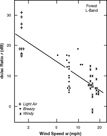
FIGURE 6.17 LCE measurements showing ratio of dc to ac spectral power vs wind speed in L-band windblown forest clutter spectra.

FIGURE 6.19 Phase One measurements showing ratio of dc to ac spectral power vs radar frequency under windy conditions at three forested sites.
In measured clutter spectra from windblown trees, not only does the maximum spectral power almost always occur in the zero-th Doppler bin, but high spectral power levels are also often resolved in neighboring Doppler bins that are very near but not right at zero Doppler. Hereafter, such near zero-Doppler spectral power is called quasi-dc power. The near zero-Doppler regime of quasi-dc power is usually 0 < |v| < 0.25 m/s. Excess quasi-dc power exists in the quasi-dc region when the spectral power initially decays rapidly but continuously from the peak power level right at zero Doppler at a rate much faster than the exponential rate evident at lower power levels in the spectral tail. The spectral power that is resolved in the zero-th Doppler bin in such spectra comes from relatively motionless parts of the tree trunks near ground level as well as from the ground surface itself, whereas the spectral power resolved as quasi-dc comes from higher parts of tree trunks and major limbs flexing slightly at very slow rates. Including the excess quasi-dc spectral power as part of the ac spectral power degrades the goodness-of-fit of the exponential shape function in the spectral tail. That is, in these circumstances even though the value of β in Eq. (6.2) is correctly selected to match the relative shape Pac(v) in the spectral tail, the value of r will be too low, with the result that the absolute level [1/(r + 1)]Pac(v) will be too high. Furthermore, to the extent that windblown clutter statistics are nonstationary, besides being too high, this level can also be dependent on the length of coherent processing interval (CPI) employed.
Therefore, in what follows, where excess (above the approximating exponential) quasi-dc power occurs in the data, it is included with the Dirac delta function as dc power in the model. This approach to quantifying dc/ac ratio r has been followed in the processing underlying the statistics upon which Eq. (6.2) is based (see Section 6.4.2). The major consequence of this approach is that the preceding spectral model approximates the exponential spectral tail region correctly, in both relative shape and absolute level, and independently of the length of CPI employed. Examples of windblown forest clutter spectra containing excess quasi-dc power are presented subsequently, as well as examples of desert and cropland clutter spectra in which a dc component from the absolutely stationary underlying ground surface (as opposed to the moving vegetation) exists as a discrete delta function.
6.2.3 MODEL SCOPE
Equations (6.1), (6.2), (6.3), and (6.4) constitute a simple but complete empirical model for characterizing the complex physical phenomenon of radar ground clutter power spectra from windblown trees based on extensive measurements. Total backscattered clutter power is represented including both dc and ac spectral components. The test of any model of a physical phenomenon is the degree to which it generally represents the phenomenon while avoiding complicating detail. The important parameters incorporated in the model of Eqs. (6.1), (6.2), (6.3), and (6.4) are wind speed and radar frequency; others that might be thought to strongly influence clutter spectra from windblown trees, but which appear to be generally subsumed within the ranges of statistical variability over the relatively large cell sizes utilized in the measurement data, include: (a) the types of trees involved (species, density, growth stage), (b) season of the year (e.g., leaves on vs leaves off), (c) wind direction, (d) polarization, and (e) angle of illumination.
It is not possible to generalize information for dc/ac spectral power ratio r for all possible varieties of vegetated (or partially vegetated) ground clutter cells from which significant proportions of backscattered clutter power come from stationary scattering elements. Subsequently discussed Lincoln Laboratory measurements of clutter spectra in scrub desert, rangeland, and cropland terrain, although indicating much larger values of dc/ac spectral power ratio when compared with forest terrain, also indicate that the residual ac spectral shape function Pac(v) is similar to that of forest. Thus the spectral model of Eqs. (6.1), (6.2), and (6.3), although explicitly derived for windblown trees, may be considered generally applicable not only to forested cells but also, at least as a first-order approximation, to cells in partially open or open terrain (desert, rangeland, cropland) as long as the value of r is increased appropriately. However, Eq. (6.4) specifying r was derived only from forested cells, and only some particular examples are provided in what follows indicating how r increases for cells incompletely filled with trees or in open agricultural terrain.
Although the exponential spectral shapes Pac(v) in Figure 6.1 are modeled to be invariant with radar frequency and vegetation type, two important ramifications are: (1) modeled widths of clutter frequency spectra Pac(f) increase linearly with radar frequency from VHF to X-band, and (2) increasing values of dc to ac ratio r in increasingly open terrain (desert, cropland) and/or with decreasing radar frequency cause absolute ac power levels [1/(r+1)] Pac(v) to decrease even though the Pac(v) shape function itself remains invariant under such circumstances.
An important requirement in the development of the current model was that its predictions of spectral extent be in the correct general Doppler regime at spectral power levels 60 to 80 dB down from zero-Doppler peaks. Much uncertainty has existed concerning the location of this regime. The extensive Lincoln Laboratory database of windblown clutter spectral measurements, without exception, indicates ever increasing rates of spectral decay (i.e., downward curvature) with decreasing spectral power level as observed on log-Doppler velocity axes such that maximum spectral extents 60 to 80 dB down are limited to Doppler velocities of 3 to 4 m/s. The exponential shape function properly reflects this important fundamental feature of the measurements. The exponential model for Pac(v) provides windblown clutter spectra wider than Gaussian as required by experiment and supported by theory [29].
An alternative popular spectral shape function Pac(v) has been power-law [10]. The measurement data clearly indicate that observed rates of decay modeled as power law at upper levels of spectral power do not continue as power law to lower levels of spectral power but fall off much faster at the lower levels. In contrast, an exponential representation generally captures, at least approximately and occasionally highly accurately, the major attributes of the windblown clutter ac spectral shape function over the entire range from near the zero-Doppler peak to measured levels 60 to 80 dB down.
The exponential model for Pac(v) is validated in Section 6.5 (see also [30, 31]) by showing that the differences in matched filter and clutter cancellation system performance between using actual measured in-phase (I) and quadrature (Q) Phase One clutter data as input to the processors, and modeled clutter spectral data of various spectral shapes (viz., Gaussian, power law, and exponential), are minimized when the spectral model employed is of exponential shape. Section 6.5 also evaluates the impact of using the exponential model for Pac(v), as opposed to Gaussian and power-law models, on the prediction of detection performance of airborne and ground-based surveillance radar using coherent adaptive processing [32, 33].
6.3 MEASUREMENT BASIS FOR CLUTTER SPECTRAL MODEL
6.3.1 RADAR INSTRUMENTATION AND DATA REDUCTION
Lincoln Laboratory has measured and characterized ground clutter power spectra over wide spectral dynamic ranges using the Phase One and LCE (L-Band Clutter Experiment) instrumentation radars [21, 25]. Both of these radars were conventional analog coherent radars. These two radars are first mentioned in this book in Chapter 1, Section 1.3. The Phase One radar and its program of clutter measurements are subsequently described more completely in Chapter 3.
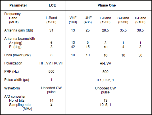
Important system parameters of these two radars are shown in Table 6.2. As shown in the table, the Phase One radar operated in five frequency bands, whereas the LCE radar operated at L-band only. With both radars, the basic type of clutter experiment suitable for examining temporal and spectral characteristics of ground clutter was the long-time-dwell experiment (see Section 3.2.2) in which relatively long sequences of pulses at low pulse repetition frequency (PRF) were recorded over a contiguous set of range gates with a stationary antenna beam. Each radar activated one combination at a time of frequency, polarization, and pulse length for any particular long-time-dwell clutter experiment. Many of the Phase One clutter spectra shown in Chapter 6 are from long-time-dwell data collected at Katahdin Hill, a forested site in eastern Massachusetts, during April and early May before leaf emergence on deciduous trees. The forested cells from which backscatter was measured at Katahdin Hill are typical of the eastern mixed hardwood forest (oak, maple, beech) with occasional occurrences of conifers (hemlock, pine), all generally 50 or 60 ft high. For the Katahdin Hill measurements, general wind conditions in the neighborhood of the principle cells from which backscatter was recorded were taken from weather information continuously broadcast from a nearby airfield. At other sites, wind conditions were measured by anemometers located at the radar site and, in many instances, also in the clutter measurement sector.
The LCE radar was a major upgrade at L-band only of the Phase One measurement equipment with substantially reduced phase noise levels [34, 35]. A primary design objective of the LCE radar was to achieve low enough phase noise such that the low-frequency Doppler components of windblown clutter could be measured to levels ≈ 80 dB below the dc or stationary component of the clutter at zero-Doppler. This objective was met by using a combination of low phase-noise local oscillators (viz., Hewlett-Packard models 8662A and 8663A) locked to a common source, a low phase-noise transmitter, and system clocks with low jitter. The transmitter used two planar triodes (viz., Eimac Y-793F) in a grounded-grid amplifier configuration providing inherently low noise sensitivity [36]. The LCE radar receiver achieved high dynamic range through careful gain distribution and proper choice of mixers and amplifiers, with particular attention paid to maintaining overall system linearity. The two channels of the analog in-phase and quadrature (I/Q) detector, which operated at a receiver IF of 3 GHz, were balanced to within approximately 0.1 dB in amplitude and 1 degree of phase. This balance provided approximately 40 dB of image rejection. The receiver baseband I/Q outputs were digitized by 14-bit analog-to-digital (A/D) converters chosen for their linearity and speed (i.e., maximum clock speed = 10 MHz). The I/Q detector dc bias was temperature-regulated to approximately 100 μV variation (i.e., to less than the least-significant bit of the A/D converter).
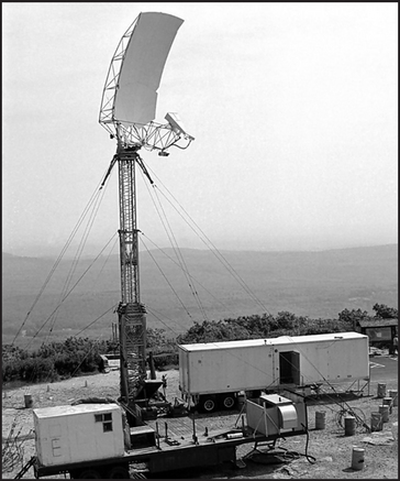
Many of the LCE clutter spectra shown in Chapter 6 are from long-time-dwell data collected at Wachusett Mountain, Massachusetts, 32 miles west of Katahdin Hill, with similar tree cover. A photograph of the LCE radar on Wachusett Mountain is shown in Figure 6.3. Another LCE measurement site was in Nevada, where backscatter data were recorded from sparse scrub vegetation typical of the western desert. In contrast with Phase One, the LCE radar could measure both the copolarized and the cross-polarized returns, although not simultaneously. For LCE clutter measurements at Wachusett Mountain, wind conditions were measured simultaneously with the clutter measurements at 10-s update intervals with an anemometer stationed on top of a 75-ft tower in a treed clutter cell along one of the three azimuth positions selected for clutter measurements. These measurements were performed in August with the deciduous trees fully in leaf.
6.3.1.1 SPECTRAL PROCESSING
LCE long-time-dwell clutter data were acquired with a stationary antenna over 70-s data recording intervals called experiments. Each LCE experiment involved the recording of 80 I and Q sample pairs per pulse repetition interval (PRI) at 2- MHz sampling frequency (i.e., 75-m range gate spacing), leading to a 6-km total recorded range swath. Clutter experiments were usually taken in sequential groups covering the various LCE polarization combinations. Phase One long-time-dwell clutter data were acquired similarly to LCE data. Table 6.3 provides the specific Phase One clutter data acquisition and spectral processing parameters applicable to the Phase One spectral results shown herein from Katahdin Hill.

All the LCE clutter power spectra shown subsequently were computed directly as fast Fourier transforms (FFTs) of the sampled temporal pulse-by-pulse return, including the dc component. A four-term Blackman-Harris window function was utilized, with highest sidelobe level at −92 dB [37]. Each temporal record of 30,720 pulses (first 61.44 s of each 70-s experiment) was divided into contiguous groups of 5,120 samples; a 1,024-point complex FFT was generated for each group by utilizing every fifth pulse; and the amplitudes of the resultant set of FFTs were arithmetically averaged together in each
Doppler cell to provide the spectrum illustrated. Thus each LCE spectrum shown is the result of averaging six individual spectra (each from a 1,024-point FFT) from an overall record of 1.024-min duration, using an effective 10-ms PRI and an effective 100-Hz PRF. The CPI for each FFT was 10.24 s.
Table 4.10 in Chapter 4 indicates that the typical correlation time for windblown trees at L-band is ∼ 1 s (see also Table 6.3). Thus the CPI utilized in LCE spectral formation, usually being ∼ 10 times the correlation time, is more than adequate to allow the random process to fully develop. The Phase One clutter spectra shown were computed similarly to the LCE spectra. Table 6.3 provides the particular Phase One spectral processing parameters utilized in generating the Phase One clutter spectra from Katahdin Hill. Table 6.3 includes both the CPI (i.e., time dwell per FFT) used and the typical correlation time of windblown trees for each Phase One frequency band, as specified by Table 4.10. These numbers indicate that the CPI covers many correlation periods at each of the five Phase One radar frequencies.
6.3.1.2 SYSTEM STABILITY
For a steady target, the spectral processing of either the Phase One or LCE radar yields a very narrow spectrum containing only dc power at zero-Doppler velocity. Figure 6.4 shows results from such steady targets. Figure 6.4(a) shows the measured LCE clutter spectrum from a desert terrain cell under very still (0 mph) wind conditions. Figures 6.4(b) and (c) show measured Phase One spectra from a large municipal water tower at L- and X-bands, respectively; in each case, clutter from trees in the same cell as the water tower just begins to broaden the spectrum near the base of the water-tower dc spike. Figure 6.4(d) shows the measured Phase One VHF spectrum from a cell containing tall grass; the windblown motion of the grass is indiscernible in this VHF measurement. In all these results, the width of the dc spectral component from the steady target is essentially the limit of spectral resolution provided by the Blackman-Harris window function, which is cleanly maintained over the full spectral dynamic range of the radar down to the system noise level (i.e., 71 to 77 dB down for Phase One, 80 dB down for LCE). The window function sidelobes occur below the noise level of either system.

6.3.1.3 SPECTRAL NORMALIZATION
Chapter 6 shows measured clutter spectra normalized to compare with analytic representations of clutter spectral density. The first step in spectral normalization is to convert the FFT output from power per spectral resolution cell to power/(m/s) so as to be directly comparable with analytic spectral shapes defining continuous density functions. This conversion is performed by dividing each point in the FFT velocity spectrum by the width of the Doppler velocity resolution cell Av. The Doppler velocity resolution cell is wider than the sampling interval by a factor equal to the equivalent noise bandwidth ENBW of the window function. Thus Δv = (λ/2) ·(PRF/N) ·ENBW, where N is the number of points in the FFT. For the four-term Blackman-Harris window used here, ENBW = 2.004 [37]. The second step in spectral normalization is to bring the power in the measured spectrum to unity for comparison with analytic spectral shapes for which the integral over the entire velocity domain is unity. In some circumstances, total power in the spectrum is brought to unity by dividing each spectral point by total spectral power. In other circumstances, where concern is only with the ac spectral shape and not the particular amount of dc power present, the ac power in the spectrum is brought to unity by dividing each spectral point by total spectral power times 1/(r + 1).
6.3.1.4 SPECTRAL POWER
Total, dc, and ac spectral power were computed in the time domain for the Phase One and LCE spectral results. Total power over the temporal record of each FFT is 1/N times the sum of the squares of the I and Q samples of received power. The dc power over the same temporal record is the square of 1/N times the sum of the I samples plus the square of 1/N times the sum of the Q samples (i.e., coherent sum). The ac power over the same temporal record is total power minus dc power. These computations were performed over each FFT contributing to each spectrum. The final time-domain quantities for total, dc, and ac spectral power are each means of the resulting set of values, one value per FFT, applicable to each spectrum.
The dc power obtained by summing coherently over a temporal record of backscatter from windblown trees depends on the length of the record (the CPI) over which the summation is performed. If the random process were well behaved (i.e., stationary), the coherent sum would converge and be largely independent of record length for lengths much greater than the correlation period of the process. However, windblown clutter backscatter records are not rigorously stationary. The statistics of the process sometimes appear to be characterized as intervals of stability separated by abrupt transitions from one stable state to another. Such abrupt changes can be caused, for example, by large tree limbs suddenly shifting position. Because the coherent sum does not always converge, the ratio of dc/ac power computed in the time domain is dependent on CPI duration.
Table 6.4 provides two examples of the dc/ac ratio obtained as a function of CPI duration for two LCE long-time-dwell backscatter measurements from cells containing windblown trees, one taken under very light wind conditions and the other under very windy conditions. The correlation times for these two experiments are estimated to be ∼ 4 s for the light-air data and ∼ 1 s for the windy data. The clutter spectra from these two measurements are discussed in Section 6.3.2.1. It is evident that a significant dc component exists in the light-air data in Table 6.4 and very little dc power exists in the windy data. The results in the table may be interpreted in terms of decreasing sampling bandwidth of the zero-velocity Doppler filter with increasing CPI, where sampling interval bandwidth is given by λ/(2 × CPI). Because no weighting is employed in these time-domain computations, the filter has a sin x/x response.
TABLE 6.4
Variation of dc/ac Ratio with Length of CPI for LCE Clutter Measurements from Windblown Trees

In the frequency domain, the zero-th Doppler bin can contain both a singular dc power component existing as a discrete delta function and ac power existing as a continuous density function. The ac power in the zero-th Doppler bin decreases with increasing resolution (i.e., with increasing CPI duration), whereas the singular dc component is theoretically independent of resolution. However, in all the measured clutter spectra shown here, normalization (division) of power/cell by Δv was performed for all cells, including the zero-Doppler cell. First-order credibility checks of the reasonableness of dc/ac ratios provided herein for spectra containing strong dc components (i.e., strong dc spikes, for example, in desert or cropland or at VHF) should therefore be performed by first decreasing the height of the spike by |Δv| dB before estimating the resultant dc/ac ratio. Note that the peak spectral level at zero Doppler (before or after division by Δv) is not itself used in any direct way in Chapter 6 to normalize measured spectral data (measured spectra are never simply aligned by peak level).
One reason that the zero-Doppler cell is not normalized differently from others is to maintain the relative shape of the raw FFT before normalization (whatever is done to one cell is done to all cells). Another reason is that the power in the zero-Doppler cell of windblown foliage spectra is often not dominated by a singular dc (i.e., delta function) component, in which circumstances the continuous power in the zero-Doppler cell requires normalization by Δv similarly to all other Doppler cells. Excess quasi-dc power in Doppler resolution cells near the zero-Doppler cell is included as dc power in computing the dc/ac power ratio used as spectral modeling information in spectra where excess quasi-dc power exists. The dc/ac ratio in which the excess quasi-dc component is included in the singular dc term is obtained in the frequency domain by best-fitting the spectral tail at high Doppler velocities with an exponential ac shape function. The excess quasi-dc power is that which exists above the approximating exponential in cells of very low Doppler velocity close to zero Doppler. The fitting process is largely independent of spectral resolution as long as the resolution is adequate to define the exponential spectral tail. As a result, the dc/ac ratio used herein, which is that required for the ac exponential shape function to match the measured spectral tail both in relative shape and in absolute level, is also largely independent of CPI duration and spectral resolution. This fitting process is discussed in Section 6.4.2.
6.3.2 MEASUREMENTS ILLUSTRATING AC SPECTRAL SHAPE
6.3.2.1 VARIATIONS WITH WIND SPEED
Figures 6.5–6.7 are examples of LCE-measured windblown forest clutter spectra under windy, breezy, and light-air conditions, respectively. The data in these figures are normalized to show ac spectral shape Pac(v) plotted against a logarithmic Doppler velocity axis similar to the modeled curves of Figure 6.1. Each figure compares the measured ac spectral shape with several exponential shape functions of various values of shape parameter β. In Figure 6.5, the measured data follow the exponential curve of shape factor β = 5.2 remarkably closely over the full spectral dynamic range shown. This match of measured ac spectral shape with exponential is among the best in the Lincoln Laboratory database, although other examples exist both of LCE and Phase One windy-day clutter spectra with equally good fits to exponential. Furthermore, the spectrum of Figure 6.5 is among the widest measured; its shape factor β = 5.2 is the basis of the “worst case, windy” specification in Table 6.1 and Figure 6.1.

FIGURE 6.6 Approximate exponential decay in a forest clutter spectrum measured under breezy conditions.

FIGURE 6.7 Approximate exponential decay in a forest clutter spectrum measured under light wind conditions.
Also shown in Figure 6.5 is a narrower Gaussian spectral shape function. The particular Gaussian shape shown corresponds to Barlow’s [7] much-referenced 20-dB dynamic range historical measurement (see Section 6.6.1.1). It is evident in Figure 6.5 that the overall rate of decay in the LCE data is much more exponential than Gaussian in character. Thus these LCE data support the general consensus of agreement subsequently arrived at [10–20, 27, 28] of spectral tails wider than Gaussian in windblown clutter spectra. Li [19] explains that tails wider than Gaussian are theoretically required by branches and leaves in oscillatory—as opposed to merely translational—motion.
The LCE spectral data of Figures 6.6 and 6.7 indicate that measured ac spectral shapes remain reasonably well represented by exponential shape functions under less windy conditions, with increasing values of exponential shape factor with decreasing winds (i.e., β = 8 for breezy conditions, β = 12 for light-air conditions). The results of Figures 6.6 and 6.7 are representative of many similar spectra measured in other cells on other days. Recall that normalization to Pac(v) requires raising the Ptot(v) spectrum by 10 log10 (r + 1) decibels on the vertical ordinate. The value of r applicable in Figures 6.5, 6.6, and 6.7 is 0.7, 18.9, and 29.8 dB, respectively. It is evident in Figures 6.6 and 6.7 that the measured data begin to depart from the approximating exponentials for v < 0.2 m/s as they begin to rise into the quasi-dc region, contributing to the large values of r in these data. As the amount of dc spectral power increases, less spectral dynamic range is left for measuring the ac power in the spectral tail, indicated by the rapidly rising effective system noise levels with respect to Pac(v) as wind speed decreases and dc/ac ratio increases in Figures 6.5–6.7.
As discussed later (Sections 6.6.1 and 6.6.2), power-law spectral tails plot as straight lines in plots of 10 log10P vs log10v such as those of Figures 6.5–6.7. Thus a power law of shape n = 3 (30 dB/decade) fits the data of Figure 6.6 reasonably well down to the Pac = −20-dB level.
However, this n = 3 power law cannot be extrapolated to lower levels. The local power-law (local slope tangent to the data curve) rate of decay in Figure 6.6 strongly increases (to n = 6 or 7) at the lower spectral power levels in Figure 6.6. Likewise, at first consideration, an n = 4 power law (40 dB/decade) might be thought to be a reasonable match to the measured data of Figure 6.7. The apparent goodness of this straight-line fit to the data in Figure 6.7 is heightened by the data beginning to rise above the exponential in the low-Doppler quasi-dc region v < 0.2 m/s and by the data flaring away from the exponential toward the noise level as they become limited in signal-to-noise (S/N) ratio when approaching to within 10 dB of the noise floor at higher Doppler velocities around 1 m/s. However, these two effects tend to obscure a more fundamental exponential-like rate of decay (increasing local tangent slope with decreasing power level) as shown in the region 0.2 < v < 0.7 m/s in Figure 6.7, and the upper-level power-law rate of decay can no more be extrapolated to lower levels in the light-air data of Figure 6.7 than in the windier data of Figures 6.5 and 6.6. To do so would lead to physical implausibility as the upper-level light-air power law would extrapolate to lower-level ac power levels (e.g., Pac = −60 dB) exceeding in spectral width those measured under windy conditions at the same lower levels.
Not all the Phase One and LCE clutter spectra measured under breezy and windy conditions are as closely exponential as the measured spectrum in Figure 6.5. However, like that spectrum, they all demonstrate increasing downward curvature (convex from above) with increasing Doppler velocity and decreasing power level as their most characteristic general feature in plots of 10 log P vs log v such as that of Figure 6.5. The main reason the exponential form is used herein for modeling clutter spectral shapes is that it, too, when plotted as 10 log P vs log v, possesses this increasingly downward curving shape (see Figure 6.1) while remaining wider than Gaussian as required by the measured data (see Figure 6.5). In contrast, the spectral tails of power-law functions do not have increasing downward curvature on 10 log P vs log v axes but plot linearly (i.e., extrapolate rapidly to excessive spectral width) on such axes. This matter is further discussed in Sections 6.6.1 and 6.6.2.
Most of the Phase One- and LCE-measured clutter spectra are not completely and precisely representable by any simple analytic function over their full spectral ranges. Many of these measured spectra are somewhat wider than exponential (i.e., are concave from above in 10 log P vs v plots), but they are almost always much narrower than power law (i.e., are convex from above in 10 log P vs log v plots). In such circumstances, absorbing excess quasi-dc power in the dc term usually gives the exponential model the flexibility to match the relative shapes and absolute levels of the measured spectra over extensive spectral tail regions.
Gale Force Winds (Scaled Estimate). Figure 6.8 shows a different set of three LCE-measured windblown-forest clutter spectra under light-air, breezy, and windy conditions, displayed as 10 log Ptot vs v. In contrast to the light-air, breezy, and windy spectra of Figures 6.5–6.7 (which come from three different range cells) the spectra shown in Figure 6.8 are from the same 7-km range cell on three different measurement days. These Figure 6.8 spectra clearly indicate that spectral extent from a given range cell increases strongly with increasing wind speed. In approximate measure, the data of Figure 6.8 indicate similar-sized steps of increasing spectral width for wind speeds increasing by approximate factors of 3 (from 1–2 to 6–7 mph, and from 6–7 to 18–20 mph). This observation implies that spectral width increases approximately linearly with the logarithm of wind speed [28, 38]. Such data are the basis of Eq. (6.3) specifying spectral width as a function of wind speed in the clutter model of Section 6.2. In Figure 6.8, the maximum spectral extent in the data 70 dB down from their zero-Doppler peaks is ∼ 1, 2, and 3 m/s for the light-air, breezy, and windy spectra, respectively. In these results, as ac clutter power increases and spreads out with increasing wind speed, dc clutter power decreases, as indicated by dc/ac ratios r of 0.1, −1.5, and −4.5 dB for the light-air, breezy, and windy spectra, respectively.
Figure 6.9 shows the same three spectra of Figure 6.8, now displayed as 10 log Ptot vs log v. Figure 6.9 also shows a scaled extrapolation to higher wind speeds by a further factor of 3, that is, from the 18–20 mph of the “windy” spectrum to 54–60 mph gale force wind speeds. This estimate was obtained by finite-difference extrapolation of the light-air, breezy, and windy Doppler velocities, say va, vb, and vc, to vd, the estimated gale force Doppler velocity, at multiple spectral power levels, assuming constant factors-of-3 increases in wind speed throughout. It is evident in the figure that the gale force spectral estimate is well modeled by an exponential curve of shape factor β = 4.3; this is the basis of the “typical” gale force exponential ac shape parameter specification β = 4.3 in the clutter model of Section 6.2. Increasing gale force β in this model from its typical specification based on the scaled estimate shown in Figure 6.9 to a worst-case specification of β = 3.8 brings it into very close agreement (in terms of gross spectral extent at the −14-dB level) with the only known measurements of windblown clutter under actual gale wind conditions, namely, the very early measurements of Goldstein [9] that are further discussed in Section 6.6.3.5.
6.3.2.2 INVARIANCE WITH RADAR FREQUENCY
The idea that spectral extents of windblown ground clutter Doppler-velocity spectra are in large measure invariant with radar frequency, or equivalently, that spectral widths in Doppler-frequency spectra are approximately proportional to radar frequency, has been discussed in the technical literature of the subject since the early days of radar development [6, 8, 9]. For example, early work in comparing spectral widths with radar frequency conducted at the MIT Radiation Laboratory during World War II by Herbert Goldstein and others is summarized by Goldstein’s conclusion that “The widths of the [Doppler-frequency] spectra … increase with wind speed and … appear to be essentially proportional to [radar] frequency” [8, 9]. This idea remains true in the LCE and Phase One spectral results, as indicated in Figures 6.10 and 6.11—Figure 6.10 shows VHF, L-, and X-band Doppler-velocity forest spectra under windy conditions; Figure 6.11 shows UHF, L-, and S-band forest spectra under breezy conditions.
However, the early results were mainly in the 1- to 10-cm range of wavelengths and, by today’s standards, over very limited spectral dynamic ranges (∼ 20 dB). Results such as those of Figures 6.10 and 6.11 extend the idea of frequency invariance of windblown clutter Doppler-velocity ac spectral shape over very much greater spectral dynamic ranges (> 60 dB) and to very much longer radar wavelengths [from X-band (λ = 3.3 cm) to VHF (1.8 m)]. These results are rather surprising, since the dominant, wavelength-sized scatterers at VHF (large branches, limbs) are presumably different than those at X-band (leaves, twigs). As will be shown, much more dc power exists in VHF windblown clutter spectra than at higher radar frequencies, for one reason because the VHF energy partially penetrates the foliage to reach the underlying stationary tree trunks and ground surface. As a result, the ac spectral power at VHF is measured at lower levels in the available spectral dynamic range. Still, over very many spectral measurements of windblown trees at VHF and UHF, ac spectral spreading caused by internal motion in windblown clutter generally exists at VHF and UHF at lower absolute levels of Ptot(v) but roughly equivalently in the relative shape and extent of Pac(v) to that observed in the higher, L, S, and X microwave bands.
In Figure 6.10, the VHF and X-band spectra were measured by the Phase One radar at Katahdin Hill under windy conditions on two different days in April at 2.8-km range. The L-band spectrum was measured by the LCE radar at Wachusett Mt. on 11 September at 6-km range. The Figure 6.11 spectra were all measured by the Phase One radar at Katahdin Hill also at 2.8-km range under breezy conditions in late April or early May. In general measure, the three windy-day spectra of Figure 6.10 are essentially identical in overall ac spectral shape, as are the three breezy-day spectra of Figure 6.11. Of course, temporal (minute-to-minute, hour-to-hour) and spatial (cell-to-cell, site-to-site) variability exist in LCE- and Phase One-measured clutter spectra under nominally similar wind conditions, and not all such measurements overlay one another as exactly as those shown in Figures 6.10 and 6.11. Concerning variability, even in the results of Figures 6.10 and 6.11 for which the same nominal range and azimuth apply, the spatial cells still encompass different overlapping ground areas due to the different azimuth beamwidths. Also, “… there are the usual uncertainties [because of the lack of] … simultaneity of the measurements in time” [9].
In considering possible means by which variations with radar frequency might be introduced in clutter velocity spectra, amplitude fluctuations caused by scatterer rotation and the wig-wag shadowing of background leaves by leaves in the foreground have been discussed [14, 19, 29, 39] as possible mechanisms that might complicate clutter spectra over and above phase fluctuations caused by the scatterer velocity distribution. However, one theoretical model exists [14] that incorporates scatterer rotational and shadowing effects and still provides radar frequency-independent clutter Doppler-velocity spectral shapes (i.e., “to a first approximation, the spectrum … depends only on the product λf” [14]). It is not suggested here that if multifrequency spectra could somehow be measured simultaneously from exactly the same spatial assemblage of windblown foliage, fine-scaled specific differences would not be observed in ac spectral shape with radar frequency. However, in looking across all the LCE- and Phase One-measured spectral data and the variations that exist therein, no significant trend is observed in ac Doppler-velocity spectral shape with radar frequency, VHF to X-band, as opposed, for example, to the strong trend seen in ac spectral shape with wind speed.
6.3.2.3 INVARIANCE WITH POLARIZATION
The LCE and Phase One clutter spectral data indicate that clutter spectral shape from windblown vegetation is largely independent of radar polarization, to the extent that this can be determined in non-simultaneous measurements. Figure 6.12 shows one set of three sequential LCE measurements of windblown treed-cell ground clutter spectra at VV-, HH-, and HV-polarizations obtained at approximately 2-min intervals, which are of essentially identical spectral shape. The spectral artifact in the HV-pol. spectrum of Figure 6.12 at ∼ 2.8 m/s is probably a bird. Many other LCE and Phase One VV- and HH-pol. spectra were compared from common cells selected from other sites and experiments [21]. These usually showed little or no variation in spectral shape with polarization. When variations of spectral shape with polarization did occur, such variations were usually relatively random with little evidence for the existence of any strong general effect on spectral shape with polarization.

FIGURE 6.12 Variations of LCE windblown forest clutter spectra with polarization: (a) pol. = HH, winds (mean/gusts) = 10/18 mph; (b) pol. = VV, 2 min later, winds = 13/19 mph; (c) pol. = HV, 4 min later, winds = 10/16 mph.
Other investigators have also found little effect on windblown clutter spectral shape with polarization. For example, Kapitanov et al. [13] observed that “The spectra of [X-band] echo signals from forest for different polarizations [vertical and circular] … are on the average similar.” Unpublished X-band windblown clutter spectral results obtained at Lincoln Laboratory by Ewell [20] at VV-, HH-, and circular polarizations in shrubby desert terrain also indicated no consistent differences in the spectral shapes obtained at the various polarizations.
6.3.2.4 TEMPORAL VARIATION
All LCE clutter spectra in Chapter 6 are averages of six individual 1,024-point FFTs, each formed from a 10.24-s duration temporal backscatter record. Windy-day wind conditions frequently vary considerably from one 10-s interval to the next. Such variability of windy-day conditions within a treed resolution cell from one 10.24-s interval to the next often leads to significant variability in successive individual 10.24-s dwell FFTs [21]. However, the results of Figures 6.13 and 6.14 indicate that over longer periods of 60- to 80-s, windy-day treed-cell clutter spectra can be expected to become more stationary. Figure 6.13 shows LCE treed-cell clutter spectra for three repeated experiments on a windy day, each of which is formed from an overall temporal record of 61.44 s (100-Hz PRF, 1024-point FFTs, 6 FFTs averaged). The shape of the spectrum from the first experiment is essentially identically replicated by the shape of the spectrum from a following experiment begun 65 min later, suggesting that enough averaging of wind variations occurs within 1 min to lead to some degree of convergence in average spectral shape. But wind is an extremely nonstationary dynamic random process with complex short- and long-term variation. For example, on the windy/gusty day on which the data of Figure 6.13 were collected, the gusts happened to die down over the 70-s interval covering the second experiment (begun 9 min after the first), and the spectrum formed from that data is indeed considerably narrower than the other two.

FIGURE 6.13 Variations of LCE windblown forest clutter spectra with time: Wachusett Mt., 11 September.

FIGURE 6.14 Variations of Phase One L-band windblown forest clutter spectra with time: Wachusett Mt., 22 August.
Figure 6.14 shows Phase One L-band clutter spectra for three repeated breezy-day experiments for very nearly the same treed cell at Wachusett Mt. for which the LCE data of Figure 6.13 apply. Each of these Phase One spectra is formed from a temporal record of 81.9-s duration (125-Hz PRF, 2048-point FFTs, 5 FFTs averaged). The spectrum from the first experiment is nearly identical to that of the second experiment, begun 4 min later. The spectrum from the third experiment, begun 9 min after the first, is somewhat narrower. In a similar set of five sequential experiments begun 15 min before those of Figure 6.14, the range of variability of spectral shape was similar. The slightly changing average wind conditions within 81.9-s intervals over 4- or 5-min periods resulted in only very small changes in the measured spectra, such as shown in Figure 6.14. Such results indicate that the range of variability in clutter spectra formed by averaging over 60- to 80-s data intervals under nominally similar wind conditions generally is quite low, compared with the more variable individual FFTs formed from 10- to 16-s data intervals during the same period.
6.3.2.5 EFFECTS OF SITE/SEASON/TREE SPECIES/CELL SIZE
It is not difficult to find Phase One and LCE spectra of essentially identical exponential spectral shape—two are shown in Figure 6.15. The LCE spectrum (a) measured on September 10 (leaves on deciduous trees) at Wachusett Mt. at 7.9-km range, HH-pol., 150-m range resolution, and 2° depression angle essentially overlays and replicates the Phase One spectrum (b) which was measured on May 3 (leaves not yet emerged) at Katahdin Hill at 2.4-km range, VV-pol., 15-m range resolution, and 0.5° depression angle. These two measurements were obtained with different radar receivers, and the two spectra were produced using different data reduction and processing software. Thus commonality can exist in spectral shape, in large measure because of the large cells and large degree of spatial averaging involved, despite a host of underlying differences including measurement instrumentation and parameters (range, cell size, illumination angle, polarization), site, and time of year.

FIGURE 6.15 Similar LCE and Phase One forest clutter spectra measured under windy conditions at two different sites: (a) LCE, Wachusett Mt., 10 September, and (b) Phase One (L-band), Katahdin Hill, 3 May.
The Phase One and LCE radars mimic long-range ground-based surveillance radars in the relatively long ranges, large resolution cell sizes, and low illumination angles of their measurements. Cell sizes, typically several hundred meters on a side, are large enough to encompass a large spatial ensemble of scatterers (many trees) as well as variable local wind currents within the cell. Because of the complexity of the scattering ensemble and nonuniform winds within such large cells and the temporal and spatial variability of the ensemble from cell to cell over large numbers of cells, it is difficult to discern significant site-to-site differences or significant trends with season and/or tree species in the Phase One and LCE spectral data. Other, more fine-scaled investigations, both historical [13–16] and recent [40–42], involving small illumination spot sizes (e.g., 1.8-m diameter [42]) on individual trees at short ranges (e.g., 30 m [42], 50 m [16]), provide results showing variation on treed-cell spectral shape with the type or species of trees. However, such small differences are largely absorbed within the general ranges of statistical variability in the Phase One and LCE measurements and are thus of limited consequence for the longer ranges and larger cells of surveillance radars.
From Phase One Katahdin Hill measurements acquired from a specific set of forested cells once a week over a nine-month period [21], L-band spectra were examined for seasonal variations in three wind regimes, viz., calm to light-air conditions, light-air to breezy, and windy. These results marginally showed that in each wind regime, spectral widths 60 to 70 dB down were only very slightly wider by no more than ≈0.5 m/s for summer measurements (leaves on deciduous trees) than for winter measurements (leaves off deciduous trees). An early study of Phase One spectra involved eight forested sites, four in western Canada and four in the eastern U.S. For the western Canadian sites, the dominant tree species were aspen and spruce. For the eastern U.S. sites, the forest was mixed (oak, beech, maple, hemlock, pine). Measured Doppler-velocity spectra generally showed no significant major differences in shape or extent from one forested measurement site to another, either within each group or from group to group. No significant discernible difference has been observed in the shapes of Phase One spectra from cells of 150-m range resolution compared with cells of 15-m range resolution.
6.3.3 MEASURED RATIOS OF DC/AC SPECTRAL POWER
6.3.3.1 VARIATION WITH WIND SPEED
Forested ground clutter cells contain many scatterers. Each scatterer is positioned randomly within the cell and hence produces an elemental scattered signal of random relative phase with respect to the other scatterers. Some of the scatterers, such as leaves and smaller branches, move in the wind, producing fluctuating signals with time-varying phases. Other scatterers, such as tree trunks and larger limbs, are more stationary, producing steady signals of fixed phase. The total clutter signal is the sum of all the elemental backscattered signals, both steady and fluctuating. At high wind speeds, most of the foliage is in motion, and the ratio r of dc to ac power in the clutter spectrum is relatively low. In such circumstances, and in the higher microwave bands where little foliage penetration occurs, the steady component can become vanishingly small, whereupon Eq. (6.1) simplifies to Ptot(v) ≅ Pac(v). Goldstein correctly anticipated, however, that “As the wind velocity decreases, … the steady-to-random ratio [i.e., r] would be expected to increase” [9]. Thus under light winds, a large proportion r/(r + 1) of the clutter power is at dc.
Even so, the small proportion of clutter power 1/(r + 1) that, under light winds, remains at ac can still troublesomely interfere with desired target signals. Therefore, it is necessary that a windblown clutter spectral model quantify the dc/ac ratio r expected from forested or other types of vegetated cells as a function of wind speed.
Figure 6.16 shows an LCE-measured clutter spectrum from a treed cell under very light wind conditions. The most striking characteristic of this light winds spectrum is its extreme narrowness, with spectral spreading occurring only at relatively low power levels and to relatively small extent in Doppler. This spectrum contains a large steady or dc component, and since the spectral density decays smoothly and continuously (albeit rapidly) away from the peak zero-Doppler level, it also contains high levels of quasi-dc power at very low but non-zero Doppler velocities. This spectrum may be approximately modeled utilizing a value of r = 29.8 dB, in which excess quasi-dc power is included in the dc term, and an exponential shape function for the spectral tail of shape parameter β = 12. The spectrum of Figure 6.16 is generally representative of many similarly narrow LCE and Phase One clutter spectra measured in other treed cells and on other light wind days.
Figure 8.18 An LCE windblown forest clutter spectrum measured under light wind conditions.

The particular value of dc/ac ratio r applicable to any given treed clutter cell is highly variable. Such variability is illustrated in the results shown in Figure 6.17, in which ratios of dc to ac spectral power obtained from LCE clutter measurements from many treed cells are shown as a function of wind speed. There is some difficulty in precise specification of wind speed in such results since anemometer measurements usually provide only a one-point-in-space indication of wind conditions for the total test area. Over and above the inherent variability in these data, Figure 6.17 indicates a strong trend such that the ratio of dc to ac spectral power in dB decreases approximately linearly with the logarithm of wind speed w.
8.3.3.2 VARIATION WITH RADAR FREQUENCY
Whether a scatterer in a forested clutter cell is classified as stationary or in motion depends on the radar wavelength. A back-and-forth scatterer motion of 3 cm would produce a steady signal of essentially fixed phase at VHF, but a fluctuating signal passing through all possible phases at X-band. Furthermore, at VHF and UHF, significant energy penetrates the foliage to scatter from the stationary underlying ground surface, whereas at X-band little or no energy reaches the ground. Again, Goldstein correctly anticipated that, because of such effects, the dc to ac ratio in windblown clutter spectra “… should therefore decrease with [decreasing] wavelength” [9].
Figure 6.18 shows a Phase One-measured spectrum at VHF from a treed cell under windy conditions (same spectrum as shown in Figure 6.10). It is evident in Figure 6.18 that a large dc component exists in this VHF clutter signal such that the ratio of dc to ac power in the spectrum is 14.8 dB. In contrast to the large dc component in the light winds spectrum of Figure 6.16, in which significant quasi-dc spectral power also occurs, in the lower frequency VHF spectrum of Figure 6.18 the dc component exists largely as a discrete delta function at the spectral resolution of the processing in the zero-Doppler bin. Much smaller dc components occurred in measured spectra at higher radar frequencies from the same forested cell under similarly windy conditions. Although there is a large dc component in the VHF spectrum, it also contains a significant amount of ac power of considerable spectral extent. This VHF spectrum comes from a single FFT of 61.44-s CPI (i.e., no averaging), this relatively long CPI being required to provide adequate spectral resolution at this relatively low radar frequency. The VHF spectrum of Figure 6.18 is representative of many other Phase One-measured VHF clutter spectra from other forested cells and on other windy days.
Figure 6.19 shows ratios of dc to ac spectral power vs radar frequency, VHF to X-band, obtained from Phase One clutter measurements under windy conditions at three forested sites. The solid line in the figure joins the median positions of each in-band cluster of data points; the dashed line joins the median positions of the bounding VHF and X-band clusters only. These lines indicate, over and above the inherent variability in the data, a strong trend such that the dc to ac ratio in dB decreases approximately linearly with the logarithm of the radar carrier frequency fo. Thus at X-band in Figure 6.19, virtually all the spectral power is ac, whereas at VHF the ac power occurs at levels 15 to 25 dB below the dc power. The information shown in Figures 6.17 and 6.19 substantiates the early expectations [9] in these matters. Such information was used to develop the empirical relationship given by Eq. (6.4), which relates dc to ac ratio in windblown clutter spectra with wind speed and radar frequency.
6.4 USE OF CLUTTER SPECTRAL MODEL
6.4.1 SPREADING OF σ° IN DOPPLER
Two important issues concerning the effects of ground clutter on radar system performance are the strength of the clutter, which determines how much interfering clutter power is received, and the spreading of received clutter power in Doppler. Thus predicting ac clutter power in a given Doppler cell requires predicting the backscattering clutter coefficient σ° in the spatial resolution cell under consideration (see Section 2.3.1.1), predicting the dc to ac power ratio r in the spectrum, and predicting the ac spectral shape factor Pac(v).
Let σ°trees be the clutter coefficient for windblown trees. Equation (6.1) shows that ![]() specifies the spreading of σ°trees in Doppler, i.e.,
specifies the spreading of σ°trees in Doppler, i.e.,
so ![]() represents the normalized density of windblown tree clutter power occurring at Doppler velocity v in units of [(m2/m2)/(m/s)]. For |v|>0,
represents the normalized density of windblown tree clutter power occurring at Doppler velocity v in units of [(m2/m2)/(m/s)]. For |v|>0, ![]() becomes
becomes
Let n = 0, 1, 2, …, N be the Doppler cell index, where n = 0 is the zero-Doppler cell. Then the amount of windblown-tree clutter cross section σtrees(n) that occurs in the nth Doppler cell is given by:
where σtrees(n) is in units of [m2], and fn is the Doppler frequency [Hz] in the center of the nth Doppler cell. In Eq. (6.5), Δf = Doppler cell width [Hz]; λ = radar wavelength [m]; A = spatial resolution cell area [m2]; r = ratio of dc/ac spectral power [as given by Eq. (6.4)]; and Pac(fn) is the value at f = fn of the ac spectral shape function [as given by Eqs. (6.2) and (6.3)].
Comprehensive information specifying the clutter coefficient σ°trees in Eq. (6.5) is provided in earlier chapters for the low illumination angles typical of ground-sited radar, for radar frequencies from VHF to X-band, and for both VV- and HH-polarizations, on the basis of the Phase Zero and Phase One clutter measurement databases. These clutter data are not available at cross-polarization. However, the LCE clutter data at Wachusett Mt. indicate that in forest, cross-pol. clutter coefficients are generally 3 to 6 dB but occasionally as little as 0 dB or as much as 8 dB less than the co-pol. clutter coefficients. Similar depolarization effects in forest clutter data have been observed elsewhere [13, 27, 43].
6.4.2 TWO REGIONS OF SPECTRAL APPROXIMATION
Figure 6.20 shows an idealized representation of a typical windblown clutter spectrum (solid line). As is often observed in measured clutter spectral data, this representation consists of two distinct regions, namely, a quasi-dc region near zero-Doppler velocity and an ac spectral tail region at greater Doppler velocities. Also shown is a spectral model (dashed lines) as given by Eq. (6.1). The model uses a delta function at v = 0 to represent the dc spectral component and the exponential shape function as given by Eq. (6.2) to represent the ac spectral tail. In a plot of 10 log10 Ptot vs v such as that of the figure, the exponential shape plots as a straight line of slope 4.34 β (where 4.34 = 10 log10 e and e = 2.718 …). Also, both the data and the model in Figure 6.20 are normalized to unit total spectral power, i.e.,
In these circumstances, the model is matched to the data as follows: first, β is selected so that the slope [i.e., dB/(m/s)] of the model matches that of the data in the ac spectral tail region. Next, the value of dc/ac ratio r in the model is assigned to provide a y-intercept [1/(r + 1)](β/2) so that the exponential model overlays and matches the ac region of the data in absolute power level Ptot (v) (i.e., vertical position) as well as slope. Because of the normalizations involved, this procedure results in the excess power from the quasi-dc region of the data being included in the dc Dirac delta function term [r/(r + 1)]δ(v) of the model, where excess quasi-dc power means the power in the quasi-dc region of the data that exists above the approximating exponential of the model.

Figure 6.21 shows four examples of measured windblown clutter spectra presented as 10 log Ptot(v) vs v to illustrate quasi-dc and ac spectral regions in actual measured data. Figure 6.21(a) shows an LCE spectrum; Figures 6.21(b) through (d) show Phase One spectra at L-, X-, and UHF bands, respectively. Each spectrum has an approximating exponential model shown as a straight line through the right side of the data. Each spectrum in Figure 6.21 contains excess power above the approximating exponential in a quasi-dc region near zero-Doppler. The resolution in these spectra is very fine (≈ 0.01 m/s, see Table 6.3), so in each case quasi-dc spectral power is resolved at levels well above the zero-Doppler window function limiting resolution. It is evident that absorbing the excess quasi-dc power of the data in the delta function dc term of the model in such results allows extremely good fits of the ac spectral tail regions with exponential shape functions over regions of wide Doppler extent in the spectral tails.

FIGURE 6.21 Highly exponential decay in four measured windblown forest clutter spectra: (a) LCE; (b), (c), and (d) are Phase One L-, X-, and UHF bands, respectively. Regions of excess quasi-dc power are also indicated.
As computed directly in the time domain, the zero-Doppler cell contains relatively little dc power compared with the total ac power from all the non-zero Doppler cells, for each of the examples shown in Figure 6.21. However, the quantity rmodeled increases compared with rmeasured as a result of absorbing the excess quasi-dc power in the modeled dc term. For the spectra of Figure 6.21, the values used for rmodeled are 0.7, 4.3, 2.9, and 8.0 dB for spectra (a), (b), (c), and (d), respectively. Use of these values causes the exponential straight-line fits to the data in the examples of Figure 6.21 to be shifted downwards by 10 log (rmodeled + 1) − 10 log (rmeasured + 1) decibels, resulting in the exponential models overlaying the measured data in these examples throughout the extensive ac spectral tail regions [25]. Equation (6.4) which specifies rmodeled was developed from data in which excess quasi-dc power was absorbed in the dc term to gain the benefit of improved fidelity in modeling spectral tails.
No simple ac model (i.e., analytic expression), including exponential, can adequately represent both the quasi-dc region |v| < 0.25 m/s and the ac region |v| > 0.25 m/s of the data in Figures 6.20 and 6.21. The objective of Chapter 6 is realistic representation of the ac region or spectral tail of the data. Even the simplest single-delay-line MTI filter can usually sufficiently reject dc and quasi-dc clutter power in the region |v| < 0.25 m/s. It is the tail of the clutter spectrum that requires definition to enable, for example, knowledgeable design of the skirts of MTI filter characteristics or other Doppler signal-processing ground clutter rejection techniques in the region |v| > 0.25 m/s (see Section 6.5). In the modeling information provided herein, excess quasi-dc power is included in the dc term in situations where including it as ac power would degrade representation of the ac spectral tail. Users of this information whose interests in clutter spectra may differ from those just stipulated need to be aware that some of the dc power in the delta function of the current model is often spread slightly into a near-in quasi-dc region |v| < 0.25 m/s in actual measurements. As an alternative to absorbing the excess quasi-dc power in the dc delta function, the quasi-dc region in each specific measured clutter spectrum can instead be represented by a second, very sharply declining, measurement-specific exponential function [31]. This alternative can be helpful in analysis situations in which the Dirac delta function is not of sufficient analytic tractability.
6.4.3 CELLS IN PARTIALLY OPEN OR OPEN TERRAIN
6.4.3.1 DESERT
Ground clutter spatial resolution cells in which some of the backscattered power comes from stationary scattering elements such as the underlying terrain surface itself or large fixed discrete objects (water towers, rock faces) provide correspondingly larger values of dc/ac ratio r in the resulting clutter spectra. In the ground clutter spectral measurements conducted by the LCE radar at its desert site, portions of barren desert floor were visible between the sparse desert bushes (greasewood, creosote) typically of heights of 3 or 4 ft. Figure 6.22 illustrates a typical LCE clutter spectrum measured at this desert site under windy conditions (wind speed ≅ 20 mph). It is evident that this desert clutter spectrum contains a large dc component at zero-Doppler velocity, the result of backscatter from the stationary desert floor.

FIGURE 6.22 An LCE-measured clutter spectrum from desert terrain (scrub/brush, partially open) under windy conditions.
The ratio of dc/ac power computed directly in the time domain for the desert spectrum of Figure 6.22 is 24.1 dB. Normalization of measured spectral data to Ptot(v) involves division of power per resolution cell by the width of the cell Δv. For the data of Figure 6.22, Δv equals −16.22 dB, so this procedure raises the power in each cell by 16.22 dB. For spectra like that of this figure with a large dc component, the power in the zero-Doppler cell is not distributed over Δv but exists as a singular dc component. Reducing the zero-Doppler peak by 16.2 dB allows more straightforward interpretation of r = 24.1 dB as simply the ratio of the reduced zero-Doppler peak to the total ac power (i.e., the power level of the step function existing in the unit interval −0.5 < v < +0.5 m/s and containing the same total ac spectral power as the measured spectrum).
The desert/windy clutter spectrum of Figure 6.22 contains extensive ac spectral spreading at lower power levels. The low-level ac spectral spreading in these data is due to wind-induced motion of the desert foliage. Other LCE-measured desert spectra from similar cells under light or calm wind conditions showed little or no spectral spreading over as much as 80 dB of spectral dynamic range [see Figure 6.4(a)]. Unlike the forest/light wind spectrum of Figure 6.16, which also contains a large dc component but in which the spectral power decays rapidly but broadens continuously away from the zero-Doppler peak, the dc component in the desert/windy spectrum of Figure 6.22 exists more as a discrete delta function at the spectral resolution of the window function over the higher levels of spectral power.
Figure 6.23 shows the ac spectral tail region of the desert/windy spectrum of Figure 6.22 at higher Doppler velocities as 10 log Pac(v) vs log v. Also shown in Figure 6.23 is the forest/windy spectrum previously shown in Figure 6.5. Both measured spectra in Figure 6.23 are normalized to Pac(v). The 24-dB dc/ac ratio in the desert spectrum (a) of Figure 6.23 results in an effective 24-dB loss of sensitivity (i.e., higher noise level) compared with the forest spectrum (b) in measuring ac spectral shape. Otherwise, the ac spectral shape of the desert/windy spectrum in Figure 6.23 almost exactly overlays that of the forest/windy spectrum over their common interval of available spectral dynamic range.

FIGURE 6.23 Comparison of ac spectral shapes of LCE (a) desert (scrub/brush) and (b) forest clutter spectra under windy conditions.
It was previously shown that the exponential shape factor β = 5.2 provides an excellent match to the forest/windy spectrum of Figure 6.23. On the basis of these data, the windblown clutter ac spectral shape that applies for densely forest-vegetated clutter cells under windy conditions also applies for more open desert-vegetated cells. That is, these data suggest that the ac spectral shape function caused by windblown vegetation in a cell may be, at least to a first-order approximation, somewhat independent of the type of vegetation in the cell. However, this equivalence does not extend to include dc/ac ratio; the dc to ac ratio of clutter spectral power is much higher in partially open desert than in forest terrain.
Knolls, Utah. Figure 6.24 shows X-band desert clutter spectra measured by the Phase One radar at two western U. S. desert measurement sites—Booker Mt., Nevada, and Knolls, Utah—in summer season. At both sites these spectra were obtained as eight-gate averages, 15 FFTs per gate (2,048-point FFTs, PRF = 500 Hz, hor. pol., gate width = pulse length = 150 m). The Booker Mt. spectrum of Figure 6.24(a) was measured from barren level mud flats under calm wind conditions and light rain at 12- to 13.2-km range and 2.3° grazing angle. This Booker Mt. spectrum shows essentially no spectral spreading beyond the window-function resolution over a 60-dB spectral dynamic range (except for the small residual spur indicated at the base of the dc-spike 56 dB down), and again evidences the field capability of the Phase One radar for making X-band clutter spectral measurements at low Doppler frequencies [compare with Figure 6.4(c)].

FIGURE 6.24 Phase One X-band desert clutter spectral measurements: (a) Booker Mt., Nevada, and (b), (c) Knolls, Utah.
In contrast to no spectral spreading at Booker Mt. in Figure 6.24(a), Figures 6.24(b) and (c) show an X-band desert spectrum from Knolls with significant spectral spreading. The Knolls spectrum was measured from very level terrain containing sparse, low, desert scrub vegetation under 11- to 16-mph wind conditions at 2.5- to 3.7-km range and 0.5° grazing angle. This X-band desert spectrum, although containing a significant dc component, contains less dc power than the LCE L-band Nevada desert spectrum of Figure 6.22. As a result, more ac spectral dynamic range is available for defining the shape of the X-band desert spectrum in Figure 6.24(c) than was available for defining the shape of the L-band desert spectrum in Figure 6.23. This X-band Knolls desert spectrum [Figures 6.24(b), (c)] is very similar to other Phase One and LCE windblown clutter spectra observed at other radar frequencies and from other types of vegetation.
The basic similarities of the Knolls spectrum to other Phase One- and LCE-measured spectra are in the increasing downward curvature with increasing Doppler velocity and decreasing power level displayed in Figure 6.24(c) on 10 log P vs log v axes. This downward curvature also characterizes the exponential shape factor. Thus through a broad central region of increasing downward curvature in the data of Figure 6.24(c), the exponential shape factor β = 11.2 overlays the data and captures its general shape. At upper levels, the data rise somewhat above the approximating exponential in the quasi-dc region |v| < 0.21 m/s; this excess quasi-dc power is included as dc power in the dc/ac ratio of 5.2 dB ascribed in modeling this spectrum. The slight broadening beyond exponential at very low levels in Figure 6.24(c) as the measured data approach to within 10 dB of the noise level is partially the result of S/N limitations in this region. In contrast to the exponential shape factor generally capturing the shape of this spectrum, power-law rates of decay [Figure 6.24(c)] increase from n ≅ 2 (20 dB/decade) at upper levels to n ≅ 4 (i.e., 40 dB/decade) at intermediate levels to n > 6 (> 60 dB/decade) at the lowest levels; in other words, no single power law comes close to capturing the general shape of the X-band desert spectrum shown in Figures 6.24(b) and (c).
8.4.3.2 CROPLAND
The Phase One radar acquired clutter measurement data at the farmland site of Beulah, N. Dakota, during the first two weeks of June [44]. The open agricultural fields in the measurement sectors around Beulah were mostly in wheat; in early June, the wheat was not yet very high. Trees occurred at ∼1% to 3% incidence by area, for the most part at low-lying elevations along creekbeds. The primary Beulah measurement swath examined comprised 16 contiguous 150-m gates from 4.5- to 6.75-km range. Over this swath, the terrain was well illuminated by the Phase One radar at a depression angle of ∼ 0.4°. Windblown wheatland clutter spectra were generated for all 16 primary-swath gates at vertical polarization and pulsewidth in all five Phase One frequency bands. In each band, 2048-point FFTs were generated and averaged to form the spectrum for each gate. The effective PRF and number of FFTs averaged in each band were at X-band, 500-Hz PRF, 15 FFTs; at S-band, 167-Hz PRF, 5 FFTs; at L-band, 100-Hz PRF, 3 FFTs; at UHF, 33.3-Hz PRF, 1 FFT; and at VHF, 12.5-Hz PRF, 1 FFT. Considerable gate-to-gate variation occurred in the resultant clutter spectra.
Six particular gates (10–12 and 14–16) at longer ranges in the primary swath were selected as under strong illumination and essentially containing pure wheat fields within the azimuth main beamwidth in all bands. Spectra from these gates were averaged together in each band to provide a generalized indication of pure windblown wheatland clutter spectra.
Figure 6.25 shows the resultant generalized clutter spectra from pure windblown wheatland in all five Phase One frequency bands. These measurements were obtained on four different days under relatively windy conditions. The results show significant spectral spreading in each of the four upper bands (X, S, L, and UHF) to either side of a strong dc component. Spectral spreading in these bands extends to power levels 60 to 70 dB below zero-Doppler peaks and to corresponding Doppler velocities generally < ∼1 m/s. In contrast, the VHF wheatland spectrum shows absolutely no spectral spreading to a level 65 dB down under 12-mph winds. This complete lack of VHF spectral spreading is due to a combination of (a) a high degree of penetration of the VHF radiation through the wheat stalks to the underlying stationary ground, and (b) the amplitude of the 12-mph windblown motion of the wheat stems being < 1λ at VHF (< 1.7 m). Note that the UHF wheatland spectrum, which shows the greatest degree of spreading of any of the four upper-band spectra to a maximum Doppler velocity of ∼1.25 m/s, was measured under much windier conditions (27 mph).

FIGURE 6.25 Phase One five-frequency clutter spectra from North Dakota wheatland measured on four different days in early June under strong breezy or windy conditions.
The ac spectral spreading in the four upper-band wheatland clutter spectra of Figure 6.25 is highly exponential in shape, as indicated by the relatively linear decay displayed on the 10 log P vs v axes used in Figure 6.25. The three ac spectral shapes at S-, L-, and UHFbands are remarkably exponential, and in fact are reasonably well-fitted by the exponential shape factor β = 9, which is not out of line with the values of exponential shape parameter appropriate for windblown forest at similar wind speeds (see Table 6.1). Each spectrum also shows a strong dc component. However, the X-band spectrum in Figure 6.25 shows a much decreased dc component, such that much of the pure dc power in the lower bands has spread into a quasi-dc region |v| ≤ ∼ 0.25 m/s at X-band. The dc to ac ratios in these spectra for X-, S-, L-band, and UHF are: 4, 17, 21, and 17 dB respectively.
Beiseker, Alberta. Another agricultural site visited by the Phase One radar in summer season was Beiseker, Alberta (see Section 3.4.1.4.2). The Phase One summer visit to Beiseker was in August when the crops (mostly wheat and other grains) were mature and thus higher than for the June visit to Beulah. Figure 6.26 shows an S-band summer Beiseker cropland clutter spectrum measured as a 16- gate average of 150-m range gates at vertical polarization (5 FFTs per gate, 2048-point FFTs, PRF = 500 Hz). The PRF of 500 Hz used to make this spectrum was higher than the 167 Hz generally used at S-band, resulting in somewhat reduced spectral resolution. This Beiseker spectrum is from measurements at 10- to 12.4-km range under 7- to 12-mph winds. The measurement geometry resulted in illumination at a depression angle of ∼0.4°. The 2.4-km Beiseker measurement sector was almost entirely in mature wheat, although it was somewhat broken in places and dissected with a stream bed, resulting in small secondary incidences of herbaceous rangeland and minor scrub/brush.

The 16-gate, mature-wheat, Beiseker S-band spectrum of Figure 6.26 is well represented as exponential, although containing less dc power than the 6-gate, young-wheat, Beulah S-band spectrum included in Figure 6.25. The exponential shape factor that best represents the Beiseker spectral shape is β = 13, greater than the β = 9 Beulah value as a result of the lighter winds at Beiseker. Power-law rates of decay shown in Figure 6.26(b) increase from n ≅ 3 (30 dB per decade) at intermediate levels to n ≅ 5 (50 dB per decade) at lower levels. The dc/ac ratio in which excess quasi-dc power is included as dc power to enable the β = 13 shape factor to fit the spectral tail in Figure 6.26 is 12.2 dB.
The Beiseker 16-gate spectrum of Figure 6.26 is essentially identical in all respects to a corresponding Beulah wheatland 16-gate spectrum35 (not shown). That is, although detailed gate-to-gate differences exist in these data caused by variations in topography, crops, and wind speeds, when averaged over broad 2.4-km swaths these results indicate that exponential spectral spreading generally occurs in open cropland terrain without much site-specific variation.
de Loor’s Results. Much earlier measurements of clutter spectra from windblown crops (including wheat) made with a noncoherent X-band system were reported by de Loor, Jurriens, and Gravesteijn [45]. The one example shown by de Loor et al. is an ac spectrum for full-grown wheat under 5- to 7-mph winds of ∼ 40-dB spectral dynamic range. This spectrum appears to be highly exponential and is very similar in shape to the Phase One-measured Beulah pure-wheat spectra of Figure 6.25. Spectral widths at the −3- and −10-dB levels as a function of wind speed for winds up to 22 mph are also provided by de Loor et al. in composite plots covering four different crop types (wheat, alfalfa, sugar beets, potatoes). The maximal extent points in these results fall in closely with the predictions of the current windblown clutter exponential model at corresponding −10- and −25-dB levels under windy conditions (see Figure 6.1), after taking into account that de Loor’s results are noncoherent (i.e., wider spectra by a factor of ∼1.4, see Section 6.6.1.1). However, de Loor et al. “could not conclusively [show] significant [spectral] differences between different crop types.” Detailed comparisons of Phase One spectral results with those of de Loor et al. reinforce Phase One indications suggesting no large differences in ac spectral shape or extent at microwave frequencies between windblown tree spectra and windblown crop spectra, or indeed, between windblown crops at different stages of maturity, from different sites, and of different crop types, under windy conditions.
6.4.3.3 RANGELAND
Clutter spectral results were obtained for rangeland terrain in which patches of trees (45-ft high aspen) and patches of shrubs (15-ft high willow) occurred over open areas of herbaceous (grassy) rangeland [24, 25]. Five-frequency spectra were obtained, each averaged over 76 contiguous 15-m range gates, in which a number of FFTs per gate were also averaged. A significant dc component existed in these spectra (e.g., of dc/ac ratio as much as 15 to 20 dB), largely the result of geometrically visible open ground occurring between the patches of trees and shrubs. “Shoulders” were evident in the spectral shapes at the onset of the ac spreading just at the base of the dc spikes [cf. Figures 6.22, 6.24(b), 6.25]. Such shoulders in spectral shape have been associated with the natural resonant frequency of the trees (see Section 6.6.1.3). Beyond these shoulders, the rates of decay over the ac spectral tail regions in the rangeland spectra were highly exponential. See [25] for plots of these rangeland spectra, as well as other considerations involved in their modeling including their dc/ac ratios.
6.4.4 MTI IMPROVEMENT FACTOR
A significant advantage of an exponential spectral model for clutter is its analytic tractability. Here an example of this tractability is provided by deriving the MTI improvement factor of a single delay-line canceller operating in an environment of windblown clutter exponentially distributed in Doppler. Also derived is the single delay-line canceller MTI improvement factor that results under the more traditional assumption of Gaussian-distributed clutter, which is then compared with the improvement factor pertaining to exponentially distributed clutter. In deriving those improvement factors, the earlier approaches of Skolnik [1] and Narayanan et al. [42] are followed for deriving improvement factors for Gaussian spectral shapes. However, also explicitly included in the derivations here is the effect of the dc spectral component on the improvement factor. The expression for n cascaded delay-line cancellers operating in exponential clutter is also presented.
Note that the power-law function [see Eq. (6.18)] is not so analytically tractable as the exponential and Gaussian functions. For example, attempting to follow the preceding approach to obtain the single delay-line canceller improvement factor for power-law-distributed clutter leads to an infinite integral expression that cannot be simply evaluated analytically.
6.4.4.1 PRELIMINARY ANALYSIS
The input clutter power within one pulse repetition interval T entering the single delay-line canceller is given by

where fp = 1/T is the PRF and Ptot(f) is the total clutter spectral power density as given by Eq. (6.1) (transformed from Doppler velocity v to Doppler frequency f). Since fp must be much greater than the clutter spectral extent of Ptot(f) for successful MTI operation, the limits of integration in the preceding integral can be further expanded to ± ∞ without practical consequence on Pic, whereupon
The equivalence of the infinite integral expression to unity in this equation is required by the definition of Ptot(f) in Eq. (6.1). The frequency response function in the power domain for a delay line of time delay T is given [1] by
Thus the residual clutter power after cancellation is given by
In this equation, the sine function in |H(f)|2 may be replaced by its small-angle approximation (i.e., its argument), again because fp = 1/T greatly exceeds the practical spectral extent of Ptot(f). The result of this substitution is
The total clutter spectral power density Ptot(f) is given by Eq. (6.1) as
where r is the ratio of dc to ac power in the clutter spectrum and Pac(f) is the ac spectral shape factor. Substituting this expression for Ptot(f) into the above equation for Poc and recognizing that the term involving integration over the delta function term vanishes, the general result is that the output clutter power from a single delay-line canceller is given by
The MTI improvement factor I of the single delay-line canceller is given [1,42] by
where ![]() , the average gain of the canceller, can be shown [1] to equal 2. Therefore, I of the single delay-line canceller is given by
, the average gain of the canceller, can be shown [1] to equal 2. Therefore, I of the single delay-line canceller is given by
where Poc is given by Eq. (6.6).
6.4.4.2 EXPONENTIAL CLUTTER
Clutter distributed exponentially in Doppler frequency f is given by Eq. (6.2) as
where β = (λ/2)β and β is as specified in Eq. (6.3) or Table 6.1. It follows that
Using the standard result ![]() , the preceding equation reduces to
, the preceding equation reduces to
Representing I of the single delay-line canceller in exponentially distributed clutter as Iβ, it follows that
where vp = (λ/2)fp. Skolnik has extended Eq. (6.7) to apply to n delay line cancellers in cascade (see [1], p. 158), as:
6.4.4.3 GAUSSIAN CLUTTER
Clutter distributed Gaussianly in Doppler frequency f is given by Eq. (6.17) as
where g’ = (λ/2)2g. It follows that
Using the standard result ![]() the preceding equation reduces
the preceding equation reduces
If I of the single delay-line canceller in Gaussianly distributed clutter is represented as Ig, it follows that
Except for the inclusion of the term (r+1), which explicitly shows the effect on Ig of nonzero dc/ac spectral power ratio r, this expression for Ig is otherwise identical to that provided elsewhere [1,42]. Both Eqs. (6.7) and (6.9) reduce to
where σ is the standard deviation in the respective spectrum [i.e., in Gaussian-distributed clutter, ![]() ; in exponentially distributed clutter,
; in exponentially distributed clutter, ![]() .
.
6.4.4.4 NUMERICAL EXAMPLES
It is evident from Eqs. (6.7), (6.9), and (6.10) that I obtained in Gaussian clutter exceeds that obtained in exponential clutter by a decibel amount given by
assuming that the radar parameters λ and fp and the clutter dc/ac ratio r are the same in both cases. As a numerical example, consider Barlow’s [7] much-referenced Gaussian clutter spectrum under windy (20-mph) conditions for which g = 20 (see Section 6.6.1.1). The value of β from the exponential clutter model of Section 6.2 for similar windy (15- to 30-mph) conditions is specified in Table 6.1 as β = 5.7. Applying Eq. (6.11) using these clutter parameters shows that the single delay-line canceller improvement factor obtained in g = 20 Gaussian clutter is 3.9 dB greater than that obtained in β = 5.7 exponential clutter, independent of radar frequency and processing-specific parameters such as pulse repetition frequency. That is, the fact that exponential clutter spreads the clutter in Doppler beyond that of the more usually assumed Gaussian clutter results in a 3.9 dB loss in improvement factor.
As a further numerical example, the values of Iβ obtained by an X-band radar (i.e., λ = 3 cm) of fp = 1000 Hz operating in exponential clutter are shown in Table 6.5 as computed from Eq. (6.7). The exponential clutter for which Table 6.5 applies is that of the model of Eqs. (6.1), (6.2), (6.4) and Table 6.1 under various wind conditions.
TABLE 6.5
Improvement Factor Iβ in Exponential Clutter for an X-Band Radar (λ = 3 cm) with PRF = 1000 Hz

bFrom Equation (6.4)
cFrom Equation (6.7)
6.5 IMPACT ON MTI AND STAP
6.5.1 Introduction
The shape of the windblown radar ground clutter Doppler spectrum is important in determining the performance of target detection in ground clutter. In modern radar that operates with wide dynamic range and low noise floor, the decay of the spectral tails of ground clutter has significant impact on the detection of small moving targets. In such systems, detection performance can be clutter limited, even to relatively high Doppler frequencies. Therefore, the rate at which the clutter spectral tails decay (i.e., the spectral shape) with increasing Doppler frequency is an essential issue for the realistic prediction of detection performance.
The preceding section (Section 6.4.4) shows that the use of a realistic exponential ground clutter spectral shape causes significant loss in single-delay-line improvement factor I, e.g., 3.9 dB, compared to use of the more conventional Gaussian ground clutter spectral shape. Section 6.5 expands this previous discussion to consider the impact of ground clutter spectral shape on the prediction of detection performance of ground-based and airborne surveillance radar using modern coherent signal processing. It is shown that, with such processing, detection losses much greater than 3.9 dB can occur using incorrect clutter spectral shapes for performance prediction. The results presented summarize the work in this area of Professor Alfonso Farina of Alenia Marconi Systems, Rome, Italy, and his Italian colleagues, Professor Fulvio Gini and Dr. Maria V. Sabrina Greco at the University of Pisa and Professor Pierfrancesco Lombardo at the University of Rome, who took up the Lincoln Laboratory findings concerning ground clutter spectral shape and investigated the impact of these findings on radar signal processing techniques for target detection in clutter. What follows summarizes36 these investigations; for more extensive discussion and results describing this work, refer to the original technical journal articles [30–33].
Following subsections first review the derivation of how ground clutter spectral shape affects the performance of optimum coherent detectors, both for ground-based and airborne early-warning (AEW) surveillance radars, when such radars operate in a ground clutter environment of Rayleigh clutter amplitudes (i.e., I and Q components of Gaussian pdf). It has previously been shown in this book that temporal clutter amplitude statistics from windblown vegetation (particularly, windblown trees) indeed tend to be Rayleigh distributed—see Figure 5.A.16. The expressions for detection performance in Gaussian clutter, as discussed in what follows, can also apply to adaptive coherent detection in nonhomogeneous and nonstationary clutter environments, providing the I and Q clutter pdf’s remain Gaussian [46].
Numerical results are provided both at X-band and L-band in which the predicted performance of the MTI improvement factor I is compared between using an exponential shape for the ground clutter spectrum, as illustrated and modeled heretofore in Chapter 6, and using Gaussian and power-law shapes for the ground clutter spectrum, such as have been previously employed in the technical literature and which are defined and discussed subsequently in Section 6.6.1. This allows evaluation of the sensitivity of detection system performance prediction to the use of incorrect ground clutter spectral models. It is shown that the Gaussian shape can significantly overestimate system performance, whereas the power-law shape can significantly underestimate system performance, compared to the more correct exponential clutter spectral shape.
6.5.2 IMPACT ON PERFORMANCE OF OPTIMUM MTI
To evaluate the impact of the measured clutter Doppler spectrum on the detection performance, we proceed as follows. Consider a ground-based surveillance radar in which the radar receiver demodulates, filters the incoming narrowband waveform, and uniformly samples each pulse return, thus obtaining N complex samples ![]() spaced by T seconds, where T = 1/PRF is the PRI. The N samples are assembled into the N-dimensional vector z = zI + jzQ = [z[0] … z[N − 1]]T, where zI and zQ represent the vectors of the I and Q components, and the superscript “T” stands for “transpose of.” Assuming an exact knowledge of the clutter covariance matrix, the optimum MTI processor is a coherent linear transversal filter with complex coefficient vector w = [w1, w2, …, wN]T. To test a range cell for detection, the quantity wHz is evaluated (where the superscript “H” stands for “conjugate transpose of”), and the envelope of the result is compared to a detection threshold, thus ascertaining whether a target is present or not. The target signal is modeled by the N-dimensional complex-valued vector s = α p, where α is a complex parameter accounting for target amplitude and initial phase and pi = e j2πifT, 0 ≤ i ≤ N–1; f being the target Doppler frequency. The interference (i.e., clutter plus noise) is given by the vector d, where PC is clutter power; and PN is white noise power. The parameters that characterize the clutter interference are: the clutter to noise power ratio (CNR), the shape of the clutter spectrum, and the width of the clutter spectrum for given shape. In the results to follow, the shape of the clutter spectrum is specified to be either Gaussian, exponential, or power law; and the width of the clutter spectrum is characterized by either the one-lag autocorrelation coefficient ρ (X-band results), or by the −3-dB spectral width (L-band results). In all results, the mean Doppler frequency of the clutter spectrum is assumed to be zero.
spaced by T seconds, where T = 1/PRF is the PRI. The N samples are assembled into the N-dimensional vector z = zI + jzQ = [z[0] … z[N − 1]]T, where zI and zQ represent the vectors of the I and Q components, and the superscript “T” stands for “transpose of.” Assuming an exact knowledge of the clutter covariance matrix, the optimum MTI processor is a coherent linear transversal filter with complex coefficient vector w = [w1, w2, …, wN]T. To test a range cell for detection, the quantity wHz is evaluated (where the superscript “H” stands for “conjugate transpose of”), and the envelope of the result is compared to a detection threshold, thus ascertaining whether a target is present or not. The target signal is modeled by the N-dimensional complex-valued vector s = α p, where α is a complex parameter accounting for target amplitude and initial phase and pi = e j2πifT, 0 ≤ i ≤ N–1; f being the target Doppler frequency. The interference (i.e., clutter plus noise) is given by the vector d, where PC is clutter power; and PN is white noise power. The parameters that characterize the clutter interference are: the clutter to noise power ratio (CNR), the shape of the clutter spectrum, and the width of the clutter spectrum for given shape. In the results to follow, the shape of the clutter spectrum is specified to be either Gaussian, exponential, or power law; and the width of the clutter spectrum is characterized by either the one-lag autocorrelation coefficient ρ (X-band results), or by the −3-dB spectral width (L-band results). In all results, the mean Doppler frequency of the clutter spectrum is assumed to be zero.
The signal to interference power ratio SIRo at the output of the filter is given by:
where S = E {ssH} is the covariance matrix of the target signal and M = E {ddH} = (PC + PN) Mn is the covariance matrix of the interference d (i.e., clutter and noise). Mn is the normalized covariance matrix, i.e., [Mn]i, i = 1; i = 0, 1, …, N–1. The performance of the filter is described by the definition of clutter improvement factor I, as
where SIRi is the signal-to-interference power ratio referred to a single pulse at the input of the filter. For the optimum MTI processor (i.e., one having the weight vector w = cM−1p), the improvement factor is given by
The above discussion is applicable to the one-dimensional (1-D) ground-based case (i.e., single antenna) parameterized by f only, as opposed to the two-dimensional (2-D) airborne case (i.e., multiple effective antenna elements) parameterized by f and direction-of-arrival θ discussed in Section 6.5.3. As will be shown, Eq. (6.14) also applies to the airborne (2-D) case and to Kelly’s adaptive processor [46], for expressions of p and Mn extended to apply to these cases (see Section 6.5.3).
To obtain assigned values of probability of detection PD and probability of false alarm PFA, a specified level of SIRo at the output of the detection filter must be provided. The SIRi which is required at the input of this filter (in dB) to ensure the required performance is given by SIRi|dB = SIRo|dB − Ic(f)|dB. The improvement factor of the filter is different for any Doppler frequency, while SIRo is constant. Thus a normalized visibility plot is provided by showing [-Ic(f)|dB] for given N. In what follows, two sets of plots are used to represent performance:
(i) visibility curves: the inverse of Ic (i.e., SIRi required to leave SIRo = 0 dB) as a function of the Doppler frequency f for given N;
(i) improvement factor plots: Ic as a function of N, for given Doppler frequency f.
The visibility curve (the inverse of Ic) is a scaled (normalized) version of the required SIRi for given N as a function of target Doppler frequency necessary to provide a specific SIRo as required, for any given detector and target model, to ensure an assigned performance level (for example PD = 0.8 with PFA = 10−6), for the differing clutter spectral shapes. That is, the visibility curve allows the determination for given N of the SIRi that is required at the input of the radar detector to ensure the desired performance as given by SIRi = SIRo/Ic, where SIRo is a constant. The improvement factor plot allows the determination of the minimum number of radar pulses N for given f that is required to provide a desired value of Ic, also for the differing clutter spectral shapes.
6.5.2.1 X-BAND RESULTS (1-D)
The X-band results to follow compare optimum MTI filter performance as given by Eq. (6.14) for corresponding Gaussian and exponential windblown ground clutter spectral shapes under breezy wind conditions. The model utilized for clutter power spectral density (PSD) is that specified in Section 6.2, particularly by Eq. (6.1) which specifies Ptot(v) in terms of dc/ac ratio r and the ac shape factor Pac(v). The exponential spectral shape is modeled as specified in Section 6.2.1, particularly by Eq. (6.2) which specifies exponential spectral shape in terms of the exponential shape parameter β, β being specified as a function of wind speed (e.g., breezy, windy) in Table 6.1 and Figure 6.1. The Gaussian spectral shape is modeled as specified by Eq. (6.17) in Section 6.6.1.1, where the Gaussian shape parameter g is that required to give the same one-lag temporal autocorrelation coefficient ρ as that of the exponential spectrum under given wind conditions. This procedure is one way of normalizing the Gaussian and exponential shapes to be of equivalent extent in Doppler as a function of wind speed, the autocorrelation function being the inverse Fourier transform of the clutter power spectrum. The dc/ac ratio r in the clutter spectrum is modeled as specified in Section 6.2.2, particular by Eq. (6.4) which models r as a function of wind speed w and radar carrier frequency fo (see also Figure 6.2). In the results to follow, fo = 9.2 GHz (X-band), PRF = 1/T = 500 Hz, and CNR = 50 dB.
Figure 6.27 shows two visibility curves, corresponding to exponential and Gaussian clutter spectra under breezy conditions with dc/ac ratio r = unity, and for N = 16 coherently integrated pulses. For the exponential spectrum, β = 8 s/m; for both spectra, ρ = 0.9908, and r = 0 dB. Each curve shows the SIRi necessary to obtain PD= 0.8 and PFA = 10−6 vs normalized Doppler separation fT. Both curves decay from large required values of SIRi at low values of fT, where clutter strength is high, to bottom out at a much lower floor value of SIRi ≅ −61 dB at higher values of fT, the floor level being determined by the thermal noise limit. The curve for the Gaussian PSD decays much faster than the curve for the exponential PSD. That is, the MTI filter operating under the standard assumption of Gaussian clutter spectral shape significantly outperforms the MTI filter operating under the more realistic assumption of exponential clutter spectral shape. The loss in detection performance due to the exponential PSD is given by the signal power increase required by the disturbance with exponential PSD to match the performance of the disturbance with Gaussian PSD. It is evident in Figure 6.27 that this loss in detection performance caused by the exponential PSD is significant over a wide range in fT (i.e., for 0.05 < fT < 0.3) and at its maximum becomes as large as 15 dB. Corresponding results under windy conditions (not shown here) show larger differences in performance between Gaussian and exponential PSDs, with significant detection loss due to the exponential PSD spanning 0.07 < fT < 0.4, and becoming as large as 18 dB [32]. It is apparent that the predicted performance of the MTI processor is very sensitive to the assumed shape of the clutter Doppler spectrum.

FIGURE 6.27 Comparison of X-band visibility curves (1-D case) showing SIRi vs normalized Doppler offset fT (with SIRo = 0 dB) for Gaussian and exponential clutter spectral shapes under breezy conditions and N = 16 coherent pulses. (Results provided by P. Lombardo, Univ. of Rome. After [32]; by permission, © 1997 IEE.)
Figures 6.28 and 6.29 show improvement factor plots under assumptions of exponential and Gaussian clutter spectra, respectively (i.e., corresponding to the visibility curves of Figure 6.27). As in Figure 6.27, wind conditions for the results of Figures 6.28 and 6.29 are breezy. Comparison between the two figures indicates that, for a normalized target Doppler frequency of fT = 0.2, (i.e., well within the main clutter spectral region), to obtain Ic = −50 dB in the presence of an exponential spectrum requires the coherent integration of N = 10 pulses, while integration of only 6–7 pulses is sufficient for a Gaussian spectrum. In passing from breezy to windy conditions, the achievable improvement factor significantly degrades (i.e., under the assumption of an exponential PSD and close to zero Doppler at fT = 0.1, the loss in improvement factor in passing from breezy to windy is on the order of 9 dB [32]).

FIGURE 6.28 X-band improvement factor plots (1-D case) showing Ic vs N for breezy exponential clutter, parameterized by fT. (Results provided by P. Lombardo, Univ. of Rome. After [32]; by permission, © 1997 IEE.)

FIGURE 6.29 X-band improvement factor plots (1-D case) for breezy Gaussian clutter, parameterized by fT. (Results provided by P. Lombardo, Univ. of Rome. After [32]; by permission, © 1997 IEE.)
6.5.2.2 L-BAND RESULTS (1-D)
The L-band results that follow parallel the X-band results of the previous subsection, except that the comparison of optimum MTI filter performance [Eq. (6.14)] is now extended to include power-law—as well as Gaussian and exponential—windblown ground clutter spectral shapes. The power-law PSD is modeled as specified by Eq. (6.18) in Section 6.6.1.2; i.e., as parameterized by the power-law exponent n which typically takes on values of n = 3 or 4. Equivalent spectral extent for given wind conditions among the three spectral shapes of Gaussian, exponential, and power-law is now specified in these L-band results in terms of equal −3-dB frequency bandwidth in the three shapes, rather than specifying equal temporal correlation coefficients as in the X-band results. A further distinction is that the L-band results are provided for “windy” (as opposed to “breezy”) wind conditions, with wind speed specified at 30 mph. In the L-band results to follow, fo = 1.23 GHz, PRF = 500 Hz, and CNR = 70 dB (as opposed to 50 dB in the X-band results).
These parameters are appropriate for an L-band ground-based surveillance radar.
Figure 6.30 shows L-band visibility curves for Gaussian, exponential, and power-law clutter spectral shapes under windy conditions, for integration of N = 32 coherent pulses. For the exponential clutter PSD, the shape parameter for windy conditions is given by β = 5.7 (see Table 6.1). The Gaussian and power-law clutter PSDs have shape parameters providing equivalent −3 dB spectral width to that of the exponential PSD. The dc/ac ratio is as specified by Eq. (6.4) for w = 30 mph and fo = 1.23 GHz. As in the X-band results, the curve for the Gaussian-shaped clutter PSD decays much faster in Figure 6.30 than that for the more realistic exponentially-shaped clutter PSD. In the region fT < 0.1, performance prediction based on the exponential model requires SIRi up to 22 dB greater than that specified by the Gaussian model. In the region fT > 0.1, both Gaussian and exponential PSDs are below the thermal noise level, which determines the required SCRi ≅ − 84 dB in this region. The n = 3 power-law clutter PSD has a much higher spectral tail than the Gaussian or exponential PSDs (see Figures 6.44 and 6.55), resulting in much greater SCRi being required over the complete range 0 < fT < 0.5 to ensure the same detection performance. Performance prediction based on the n = 3 power-law clutter PSD is excessively pessimistic, compared to that based on the more realistic exponential clutter PSD. The n = 4 power-law prediction in Figure 6.30 is less pessimistic but still results in significant performance mismatch.

FIGURE 6.30 Comparison of L-band visibility curves (1-D case) showing SIRi vs normalized Doppler offset fT (with SIRo = 0 dB) for Gaussian, exponential, and power-law (n = 3,4) clutter spectral shapes under windy conditions and N = 32 coherent pulses. (Results provided by P. Lombardo, Univ. of Rome. After [33]; by permission, © 2001 IEEE.)

FIGURE 6.44 Three analytic spectral shapes, each normalized to unit spectral power. The g = 20 Gaussian curve corresponds to Barlow’s [7] measurement. The n = 3 power-law curve corresponds to Fishbein et al.’s [10] measurement. The β = 6 exponential curve represents much of the Phase One and LCE data.

FIGURE 6.55 Comparison of exponential and power-law spectral shapes: (a) linear and (b) logarithmic Doppler velocity axes.
Figure 6.31 shows L-band improvement factor plots for clutter of exponential spectral shape under windy conditions (i.e., corresponding to the exponential curve of Figure 6.30) but here showing variability with number of integrated pulses N; the results are parameterized by fT. It is apparent that for high target Doppler frequencies, a small number of pulses is sufficient to yield the best performance achievable, namely, Ic|MAX = CNR|dB + 10 log10(N); whereas for lower Doppler frequencies, larger numbers of pulses are necessary to converge to the same condition. Figure 6.32 compares improvement factor plots at fT = 0.5 and fT = 1/16, assuming corresponding Gaussian, exponential, and n = 3 power-law clutter PSDs. Unlike Ic for the Gaussian and exponential clutter PSDs, Ic for the power-law clutter PSD does not converge to the ideal performance, even at high Doppler frequencies.

FIGURE 6.31 L-band improvement factor plots (1-D case) showing Ic vs N for windy exponential clutter, parameterized by fT. Dotted curve indicates best performance theoretically achievable, given by Ic|MAX = CNR|dB + 10 log10 N. (Results provided by P. Lombardo, Univ. of Rome. After [33]; by permission, © 2001 IEEE.)

FIGURE 6.32 Comparison of L-band improvement factor plots (1-D case) for Gaussian, exponential, and power-law (n = 3) clutter spectral shapes under windy conditions, at fT = 1/16 and 1/2. (Results provided by P. Lombardo, Univ. of Rome. After [33]; by permission, © 2001 IEEE.)
6.5.3 IMPACT ON STAP PERFORMANCE
Consider an AEW radar equipped with an array of antennas with digital beam-forming capability. The detection problem is analyzed in the two-dimensional (2-D) plane of Doppler f and direction-of-arrival (DOA) θ (i.e., space-time approach [3, 4]). Assume that K channels demodulate and filter the incoming narrowband waveform received by either K antennas or K subarrays of antennas. Each channel samples the N returning pulses, thus obtaining N complex K-dimensional vectors ![]() spaced by T seconds. The N vectors are assembled into the NK-dimensional vector, z = [z1, …, zTK]T. Again, the detection problem is to determine, after the vector z has been received, whether it consists only of disturbance d, or, in addition to d, a 2-D target signal vector s is also received. The (N×K) ×1 target signal vector with Doppler frequency = f, DOA = θ, and complex amplitude = α is now defined as:
spaced by T seconds. The N vectors are assembled into the NK-dimensional vector, z = [z1, …, zTK]T. Again, the detection problem is to determine, after the vector z has been received, whether it consists only of disturbance d, or, in addition to d, a 2-D target signal vector s is also received. The (N×K) ×1 target signal vector with Doppler frequency = f, DOA = θ, and complex amplitude = α is now defined as:
where
where d is the antenna spacing. The normalized clutter covariance matrix Mc is a block Toeplitz matrix with blocks related to the antenna array elements. The elements of Mc are obtained from the space-time clutter correlation coefficient, which is usually expressed as:
where for simplicity the antenna spacing is set such that d = λ/2 = 2VT where V is the platform velocity [47, 48]. In Eq. (6.15), ρt(Δt) is the temporal correlation coefficient, which depends on the temporal displacement Δt of two sequential clutter echoes. This is the only term that depends on clutter internal motion, i.e., on the clutter spectral behavior under analysis herein, which is assumed to be of either Gaussian, exponential, or power-law shape. The term ρs(Δt + Δs/(2V)) is the spatial correlation coefficient, which encodes the decorrelation due to the combined effect of: (i) the motion of the radar platform (and thus of the different viewing angles over the scene) and (ii) the antenna pattern. Since this term depends on the spatial position of the receivers, it is a function of both the temporal displacement Δt (which follows from the differing sequential positions of the platform in flight) and the spatial displacement Δs of the antennas in the array. The optimum detector for the signal s embedded in correlated Gaussian-distributed interference is given by the same matched filter as for the 1-D case that now operates in the 2-D Doppler-DOA plane with corresponding 2-D definition of target vector and interference covariance matrix [33]. As is well known, the presence of multiple receivers, corresponding to displaced phase centers, makes it possible through space-time adaptive processing (STAP) to compensate for spectral spreading due to the platform motion, thus providing a significant improvement in detection performance [3, 4, 47].
As for the 1-D case, the optimum detector for the radar target s embedded in Gaussian distributed clutter with zero mean value and covariance matrix M is given by the filter weight vector M−1np, utilizing the 2-D definition of target vector and clutter covariance matrix. The performance parameter of interest is still Ic as specified by Eq. (6.14), which in the 2-D case is dependent on DOA θ as well as f. This same expression for Ic also characterizes the performance of a well-known adaptive detector [46] applicable to both ground-based and airborne surveillance radar designed to work in nonhomogeneous and nonstationary clutter environments [33].
For simplicity, results to follow are presented for detection of a target at antenna broadside aspect (DOA = θ = 0). Compared to the 1-D case of ground-based radar, the 2-D case of airborne radar has an extra parameter that influences detection performance, namely, the number of receivers K. In consequence, the two kinds of results, i.e., visibility curves and improvement factor plots described in Section 6.5.2, now each replicate for all possible values of K. However, it is usual in space-time processing to consider detection performance as a function of the number of degrees of freedom (DOF) given by the product N × K [3, 33, 47–49]. This product corresponds to the number of parameters that can be arbitrarily selected in the detection filter, this number having direct implication on the complexity of the required signal processor. Therefore, the results to follow compare the effect of different clutter spectral shapes on radar performance, assuming N × K = 64. As in the 1-D case, two sets of plots are also used to represent system performance in the 2-D case:
(i) visibility curves: inverse of Ic as a function of the Doppler frequency f for given N (with constant N × K = 64 and θ = 0);
(ii) improvement factor plots: Ic as a function of N (with constant N × K = 64 and θ = 0), for given Doppler frequency f.
In the generation of these plots for the airborne (2-D) case, it is necessary to quantify the spatial correlation coefficient ρs. This term is independent of clutter spectral behavior and depends mainly on the along-track antenna pattern. The results to follow assume a transmitter antenna pattern with a Gaussian main lobe and two Gaussian sidelobes, 25 and 40 dB, respectively, below the peak, and at normalized angles of 0.2 and 0.4, respectively, on both sides of the peak. These five antenna lobes are characterized by the same width, which corresponds to a one-lag spatial correlation coefficient of 0.995 [47].
6.5.3.1 X-BAND RESULTS (2-D)
The X-band results to follow compare STAP system performance (i.e., 2-D case) for corresponding Gaussian and exponential windblown ground clutter spectral shapes under breezy conditions. The same methodology for modeling the clutter spectra and the same values of radar parameters are utilized as specified at the beginning of Section 6.5.2.1 in the 1-D X-band case. Figures 6.33 and 6.34 show visibility plots for exponential and Gaussian clutter PSDs, respectively, under breezy conditions with dc/ac ratio r = unity. Various curves are shown in these two figures for different combinations of N and K, thus exchanging temporal DOF for spatial DOF. The optimum number of pulses is on the order of N = ∼16, which provides the lowest SIRi value needed to achieve assigned values of PD for fixed values of PFA. The undulations of the curve for N = 64 are caused by the two antenna sidelobes in this degenerate case of K = 1. Such undulations appear when the number of spatial DOF is so low as to allow little cancellation to be possible. Comparison between the results of Figures 6.33 and 6.34 reveals that the detection loss incurred by the airborne MTI processor in this 2-D example under the realistic assumption of an exponential clutter PSD as opposed to the more common assumption of a Gaussian clutter PSD can be as much as 10 dB.

FIGURE 6.33 X-band visibility curves (2-D case) showing SIRi vs fT (with SIRo = 0 dB) for breezy exponential clutter, parameterized by number of coherent pulses N (where N × K = 64, θ = 0). (Results provided by P. Lombardo, Univ. of Rome. After [32]; by permission, © 1997 IEE.)

FIGURE 6.34 X-band visibility curves (2-D case) for breezy Gaussian clutter, parameterized by N (where N × K = 64, θ = 0). (Results provided by P. Lombardo, Univ. of Rome. After [32]; by permission, © 1997 IEE.)
Figures 6.35 and 6.36 show improvement factor plots assuming exponential and Gaussian clutter PSDs, respectively, corresponding to the visibility curves of Figures 6.33 and 6.34. These figures indicate that for target Doppler frequencies well within the main clutter spectral region, i.e., for fT = 0.1 or 0.2, the MTI performance assuming Gaussian clutter significantly exceeds that assuming exponential clutter by amounts on the order of 8 to 10 dB for various numbers N of pulses integrated. In addition, the improvement factor Ic is much less sensitive to the number of temporal DOF N with the exponential spectrum than with the Gaussian spectrum, indicating that selection of the optimum ratio of temporal to spatial DOF depends on the assumed shape of the clutter spectrum. As in the 1-D case, in passing from breezy to windy conditions, the achievable improvement factor significantly degrades (i.e., under the assumption of an exponential PSD, and close to zero-Doppler at fT = 0.1, the loss in 2-D improvement factor in passing from breezy to windy is ≈10 dB [32]).

FIGURE 6.35 X-band improvement factor plots (2-D case) showing Ic vs log2N for breezy exponential clutter, parameterized by fT (with N × K = 64, θ = 0). (Results provided by P. Lombardo, Univ. of Rome. After [32]; by permission, © 1997 IEE.)

FIGURE 6.36 X-band improvement factor plots (2-D case) for breezy Gaussian clutter, parameterized by fT (with N × K = 64, θ = 0). (Results provided by P. Lombardo, Univ. of Rome. After [32]; by permission, © 1997 IEE.)
6.5.3.2 L-BAND RESULTS (2-D)
The 2-D L-band results to follow compare STAP system performance for different assumed shapes of clutter spectra using the same methodology for modeling the clutter spectra and using the same values of radar parameters as specified at the beginning of Section 6.5.2.2 for the 1-D L-band case. Figures 6.37, 6.38, and 6.39 show 2-D L-band visibility plots for exponential, Gaussian, and n = 3 power-law clutter PSDs, respectively, under windy conditions and for various numbers N of coherently integrated pulses as processed by the optimum space-time processor. In all three figures, the undulations in the curve for N = 64 are caused by effects of the two antenna sidelobes in this single-antenna-element case, as mentioned in the previous subsection. For the Gaussian and exponential clutter PSDs, the optimum number of pulses to provide the lowest SIRi needed to achieve assigned values of PD for fixed values of PFA is N = 8. In contrast, for the n = 3 power-law clutter PSD, the optimum number of pulses is N = 32.

FIGURE 6.37 L-band visibility curves (2-D case) showing SIRi vs fT (with SIRo = 0 dB) for windy exponential clutter, parameterized by number of coherent pulses N (where N × K = 64, 9 = 0). (Results provided by P. Lombardo, Univ. of Rome. After [33]; by permission, © 2001 IEEE.)

FIGURE 6.38 L-band visibility curves (2-D case) for windy Gaussian clutter, parameterized by N (where N × K = 64, θ = 0). (Results provided by P. Lombardo, Univ. of Rome. After [33]; by permission, © 2001 IEEE.)

FIGURE 6.39 L-band visibility curves (2-D case) for windy power-law (n = 3) clutter, parameterized by N (where N × K = 64, θ = 0). (Results provided by P. Lombardo, Univ. of Rome. After [33]; by permission, © 2001 IEEE.)
Figure 6.40 compares the Gaussian, exponential, and n = 3 power-law visibility plots for N = 8 and N = 32 together in one figure. At N = 32, the results for Gaussian and exponential clutter still show residuals of the space-time cancelled sidelobes. It is apparent in these results that a significant loss in performance (i.e., as much as 10 dB) occurs over a wide range in target Doppler frequencies (i.e., 0 < fT < 0.3) when using the realistic exponential spectrum compared to the more commonly used Gaussian spectrum. However, the additional loss in performance that occurs in utilizing an n = 3 power-law clutter spectrum is generally very much greater (i.e., as much as 30 dB) and extends over all available Doppler frequencies (i.e., 0 < fT < 0.5). That is, the predictions based on the power-law model require a very much higher SIRi at the system input to obtain the same detection performance as with the Gaussian or exponential models, and the impact of the space-time cancellation is very much lower for the power-law model due to the very slow decay of the power-law spectral tails. This slow decay also masks the effects of the antenna sidelobes at K = 2 using the power-law model, such effects being clearly evident in the corresponding results using the other two models.

FIGURE 6.40 Comparison of L-band visibility curves (2-D case) for Gaussian, exponential, and power law (n = 3) clutter spectral shapes under windy conditions, for N = 8 and 32 coherent pulses (where N × K = 64, θ = 0). (Results provided by P. Lombardo, Univ. of Rome. After [33]; by permission, © 2001 IEEE.)
Figure 6.41 shows 2-D L-band improvement factor plots for windy exponential clutter PSD corresponding to the visibility plots for exponential clutter shown in Figures 6.37 and 6.40. Since clutter PSD modeled to be of exponential shape most closely matches the measured spectral clutter data as discussed elsewhere throughout Chapter 6 (e.g., see Figures 6.5, 6.21, 6.54), the modeled results for Ic under windy conditions shown in Figure 6.41 are the best estimate of actual L-band clutter cancellation performance to be expected. The data indicate that the optimum number of integrated pulses N to maximize Ic for the various parameterized values of target Doppler frequency fT shown is usually such that N ≅K, in agreement with approximate theoretical expectations discussed elsewhere [48, 49] in this regard.

FIGURE 6.41 L-band improvement factor plots (2-D case) showing Ic vs log2N for windy exponential clutter, parameterized by fT (where N × K = 64, θ = 0). (Results provided by P. Lombardo, Univ. of Rome. After [33]; by permission, © 2001 IEEE.)

FIGURE 6.54 Two windblown forest clutter spectra for which exponential fits are compared with power-law fits: (a) LCE data, Wachusett Mt. (September) and (b) Phase One (L-band) data, Katahdin Hill (May).
Figure 6.42 compares 2-D L-band improvement factor plots for windy Gaussian, exponential, and n = 3 power-law clutter PSDs at two values of fT, viz., fT = 1/32 and 1/2. At fT = 1/32 (i.e., well within the main region of clutter Doppler extent and, in fact, quite close to zero-Doppler), the prediction based on Gaussian clutter significantly overestimates Ic (by 13 dB for N = 8 pulses) and the prediction based on n = 3 power-law clutter significantly underestimates Ic (by 10 dB at N = 8 pulses) compared to the more realistic prediction based on exponential clutter PSD. At fT = 1/2 (i.e., at the highest target Doppler frequency), the predictions for Ic based on the Gaussian and exponential models are essentially identical since the clutter for both these models is well below thermal noise at such high Doppler, with the result that the performance for these two models at fT = 1/2 is dependent only on thermal noise. In contrast, the estimated clutter cancellation performance using the n = 3 power-law clutter PSD model at fT = 1/2 is much poorer (i.e., is far too pessimistic, by 25 dB for N = 8 pulses) since the power-law clutter spectral tail is still well above thermal noise even at such high Doppler.

FIGURE 6.42 Comparison of L-band improvement factor plots (2-D case) for Gaussian, exponential, and power-law (n = 3) clutter spectral shapes under windy conditions, for fT = 1/32 and 1/2 (where N × K = 64, θ = 0). (Results provided by P. Lombardo, Univ. of Rome. After [33]; by permission, © 2001 IEEE.)
6.5.4 VALIDATION OF EXPONENTIAL CLUTTER SPECTRAL MODEL
Elsewhere, Chapter 6 (e.g., Figures 6.5, 6.21, 6.54) shows that measured shapes of windblown ground clutter Doppler spectra appear to be much more closely matched by an exponential approximation than by Gaussian (too narrow) or power-law (too wide) approximations. The preceding subsections in Section 6.5 show that large differences exist in predictions of MTI clutter improvement factor Ic between that based on what appears to be a realistic exponential clutter spectral shape and those based on more traditional Gaussian and power-law clutter spectral shapes. Compared to the exponential shape, the Gaussian shape substantially underpredicts the effects of clutter, and the power-law shape substantially overpredicts the effects of clutter. This section validates the exponential spectral model for windblown foliage by showing that the differences in improvement factor performance prediction between using actual measured I/Q data as input to the clutter canceller, and modeled clutter data of Gaussian, exponential, or power-law spectral shape, are minimized when the spectral model employed is of exponential shape.
To compare performance predictions obtained by using each of the three clutter spectral models (i.e., Gaussian, exponential, and power-law) to the performance actually obtained using measured I/Q clutter data, the following procedure is established. First, within the database of long-time-dwell clutter measurements from windblown trees, a typical experiment is selected, within which a typical clutter cell (i.e., range gate) is further selected such that the temporally-varying I/Q data from the cell are Gaussian-distributed (i.e., the clutter amplitude is Rayleigh-distributed—see Figure 5.A.16—indicative of purely windblown foliage within the cell, without significant contributions from stationary discrete sources embedded within the trees which would lead to Ricean-distributed clutter amplitudes—see Figure 4.22). The clutter Doppler spectrum from the selected cell is generated from the measured I/Q data for that cell. This measured clutter spectrum is then best-fitted [i.e., utilizing a minimum least squares (MLS) procedure] by each of the three clutter spectral models in turn, resulting in three sets of fit parameters defining theoretical clutter models of Gaussian, exponential, and power-law spectral shape. The parameters for each theoretical clutter model are used to define a corresponding clutter covariance matrix for each model. Each theoretical clutter model is then used to specify an optimum MTI matched filter such that the covariance matrix of the theoretical clutter at the filter input and the filter design covariance matrix are identical. Next, the actual measured I/Q ground clutter data from the cell under consideration is input to each of these three filters in turn, and the measured improvement factor Im is determined for each filter as the ratio between input and output clutter power. Note that, in each of the three cases, Im is based on a mismatch between the actual measured I/Q input data (which do not provide perfect Gaussian, exponential, or power-law spectral shape) and the filter (which is specified based on a theoretical clutter model of perfect Gaussian, exponential, or power-law spectral shape).
It is now necessary, in each of the three cases, to compare the measured value of Im obtained as described above using the actual measured I/Q clutter data as input to the filter with the theoretical value Ic that applies, assuming the filter is perfectly matched; i.e., assuming that the input data are synthetic data such as to give the perfect Gaussian, exponential, or power-law spectral shapes obtained by best-fitting each to the measured spectrum. Also assumed is that the temporal variation is Gaussian. In each of the three cases, Ic is given by Eq. (6.14), which assumes that the covariance matrix of the theoretical clutter at the filter input and the filter design matrix are the same. In each case, the appropriate figure of merit is the ratio ΔI of the measured improvement factor Im in the mismatched case to the theoretical improvement factor Ic in the matched case. Thus, in each case, ΔI = Im/Ic; and, in turn, ΔI|Gaussian, ΔI|exponential, and ΔI|power-law are computed for the particular clutter cell under consideration. For the specific technical details involved in carrying out these computations, refer to the original technical journal articles [30, 31, 33].
The figure of merit ΔI indicates the error in MTI filter performance resulting from the mismatch between the actual measured I/Q data and the assumption that the data are of either Gaussian, exponential, or power-law in spectral shape. The closer ΔI is to unity (i.e., 0 dB), the better that the particular clutter spectral model (Gaussian, exponential, or power-law) represents the measured clutter data in terms of the impact of the clutter data on the clutter canceller. If ΔI = unity (i.e., 0 dB), it indicates that the input I/Q clutter data provide a clutter spectral shape that is perfectly Gaussian, exponential, or power-law.
Figure 6.43 shows typical results for ΔI|Gaussian, ΔI|exponential, and ΔI|power-law, for one particular clutter cell containing windblown trees, utilizing N = 8 coherently integrated pulses. The measurement cell utilized is the 35th range cell in an X-band experiment (of HH-polarization) that was conducted at Katahdin Hill under windy conditions (20 to 30 mph). It is clearly evident in Figure 6.43 that the exponential model exhibits the lowest ΔI; i.e., for the exponential model, the predicted improvement factor Ic and the actual improvement factor Im (as obtained using the measured I/Q clutter data to feed the clutter canceller) are very nearly equal. The errors ΔI for the Gaussian model occur, as expected, at lower values of fT; at higher values of fT, the predictions based on both Gaussian and exponential clutter models transition to limitations caused by thermal noise. Also as expected, the errors in ΔI for the power-law model (of power-law exponent n = 3) occur over the full range 0 < fT < 0.5 due to the slow decay of the power-law spectral tails.

FIGURE 6.43 Differences in improvement factor (i.e., ΔI) between using measured X-band I/Q clutter data (35th range cell) as input to processor (1-D case), and theoretical clutter data of Gaussian, exponential, and power-law (n = 3) spectral shapes (each best fitted to the measured spectrum), vs normalized Doppler frequency fT, for N = 8 coherent pulses. (Results provided by P. Lombardo, Univ. of Rome, and F. Gini and M. Greco, Univ. of Pisa. After [33]; by permission, © 2001 IEEE.)
The results for ΔI shown in Figure 6.43 are generally representative of similar results for other numbers N of integrated pulses, and for data from other tested range cells and other tested experiments at L-band as well as X-band. Such results validate the exponential clutter spectral model as described in Section 6.2 as being most realistic with which to model windblown radar ground clutter spectra, and indicate that the more commonly used Gaussian and power-law models (as described hereafter in Section 6.6) are comparatively unsatisfactory. The ramifications of improvement factor prediction error ΔI to prediction error in PD and PFA are discussed in the references [30, 31, 33].