
3.6. HIGHER MOMENTS AND PERCENTILES IN MEASURED LAND CLUTTER SPATIAL AMPLITUDE DISTRIBUTIONS
The subject matter of Chapter 3 is multifrequency low-angle land clutter amplitude distributions as measured from large, repeat sector, spatial macroregions of visible terrain. Previously, the mean levels (i.e., first moments) in these distributions have been under discussion. Here, in Section 3.6, the repeat sector clutter distributions are brought under more complete description by numerically specifying their higher moments, namely, the ratio of standard deviation-to-mean (which is a normalized measure of the second moment), the coefficient of skewness (or normalized third moment), and the coefficient of kurtosis (or normalized fourth moment), and several particular percentile levels in them, namely, the 50- (or median), 70-, and 90-percentile levels. These six statistical attributes are defined in Appendix 2.C. Each of them is provided as a median value of the particular attribute over a number of repeat sectors and measurements by frequency band within the same terrain groups as in Table 3.6. Thus, these higher moments and percentiles are generalized (i.e., central) values by terrain class and radar frequency band.
Whereas the means of the clutter amplitude distributions are largely independent of resolution, the spreads in these distributions are fundamentally dependent on radar spatial resolution. As a result, all of the higher attributes presented in this section depend strongly on resolution. Therefore, in what follows, the generalized results by terrain class for higher moments and percentiles are separated, in different tables, between those applicable for the wide pulse (i.e., 150 m) and those applicable for the narrow pulse (i.e., 15 m at L-, S-, and X-bands; 36 m at VHF and UHF). In these tables, the variations with range resolution are observable by comparing and contrasting between pairs of tables, and the essential variations with azimuth resolution are observable by comparing and contrasting between different frequency bands in any given table. Many of the trends with resolution in these tables by terrain type and depression angle are carried over into the clutter models developed in Chapters 4 and 5.
The medianized results by terrain class for skewness, kurtosis, and 50-, 70-, and 90-percentiles presented in Section 3.6 are obtained somewhat differently than are the similar generalized results for means and standard deviations. The fundamental difference is that the repeat sector results for higher moments and percentiles are medianized over all the repeat sector experiments, including the day-to-day repeats of which there are nominally four per experiment; whereas, the results for mean and standard deviation are medianized over a selected subset in which only a single, centrally selected (best) experiment from each set of day-to-day repeats is included. To the extent that the repeated experiments repeat exactly (usually, a good approximation), the statistics do not change.
3.6.1. RATIO OF STANDARD DEVIATION-TO-MEAN
Values for ratios of standard deviation-to-mean in repeat sector ground clutter amplitude distributions at all Phase One measurement sites are plotted in Figures 3.45 and 3.46 for urban sites and rural sites, respectively. For each repeat sector, values are plotted for each of the 20 combinations in the radar parameter matrix (i.e., five frequencies, two polarizations, two resolutions). In Figures 3.45 and 3.46, very large values of ratio of standard deviation-to-mean are generally observed in both urban and rural terrain, resulting from the long high-side tail in these amplitude distributions caused by isolated strong returns from discrete sources over a wide range of amplitudes. In particular, in the urban data of Figure 3.45 at X-band, there is a clear-cut separation between narrow pulse and wide pulse results such that the narrow pulse data have much higher spreads than the wide pulse data; in the lower frequency bands there remains relatively good separation (i.e., little overlap) between narrow pulse and wide pulse results. Spreads in the urban data, as given by ratio of standard deviation-to-mean, are never less than ≈5 dB in Figure 3.45.

FIGURE 3.45 Ratio of standard deviation-to-mean in clutter amplitude distributions at five urban sites. Five-frequency repeat sector data.

FIGURE 3.46 Ratio of standard deviation-to-mean in clutter amplitude distributions at 37 rural sites. Five-frequency repeat sector data.
Maximum spreads in the rural data in Figure 3.46 can be approximately as large as in the urban data. The average spreads in the rural data are less than in the urban data, but minimum observed spreads in the rural data are much less than in urban data, and in a number of measurements, approach values close to unity (i.e., ratios of standard deviation-to-mean near zero dB) indicative of Rayleigh statistics.
Figures 3.45 and 3.46 separate the measured values of ratio of standard deviation-to-mean into only two terrain types, urban and rural. These values are next separated within the total 12-category set of terrain types as given by Table 3.3. Tables 3.12 and 3.13 show ratios of standard deviation-to-mean for ground clutter spatial amplitude distributions, by frequency band in all 12 terrain classes, for the Phase One wide pulse and narrow pulse, respectively. These numbers are medianized and, hence, generalized from groups of repeat sector measurements with a variable number of measurements in each group. Measurements at both polarizations are included in these groups.
The ratio of standard deviation-to-mean is the fundamental statistical measure of spread (or statistical dispersion) in the distribution. When the ratio is equal to unity, it is indicative of Rayleigh statistics. Most of the results in Tables 3.12 and 3.13 are considerably greater than unity, indicating that extreme cell-to-cell variability exists in low-angle ground clutter statistics. This variability occurs because, at angles near grazing incidence, returns are measured over a wide range of strengths from all of the vertical features rising above the mean elevation of the clutter patch.
The underlying trends observed in Tables 3.12 and 3.13 are as follows. A comparison of Tables 3.12 and 3.13 shows that the ratio of standard deviation-to-mean usually increases with increasing range resolution. In either table, a weak trend is observed where the ratio of standard deviation-to-mean tends to increase as azimuth beamwidth decreases from VHF to X-band (e.g., agricultural/high-relief; marsh/low depression angle). For a given spatial resolution (i.e., for a given frequency band in either table), the ratio of standard deviation-to-mean usually decreases with increasing depression angle. Large ratios of standard deviation-to-mean are observed in urban and agricultural terrain because these terrain types are dominated by discrete objects; smaller ratios occur in forest, particularly at high angles, and in mountains, where steep forested slopes also prevail. As angle of illumination increases in forested terrain, the phenomenon gradually transitions from a widespread Weibull regime towards a more narrowly-spread Rayleigh regime.
It is evident that these observed trends in ratios of standard deviation-to-mean in Tables 3.12 and 3.13 are less well defined than the trends in mean strength previously discussed. The more comprehensive Phase One survey data considered in Chapter 5 provide improved accuracy of such observed second-moment trends.
3.6.2 SKEWNESS AND KURTOSIS
The coefficients of skewness and kurtosis are normalized measures of the third and fourth central moments, respectively, of any distribution (see Appendix 2.C). Skewness is a measure of asymmetry in the distribution. Kurtosis is a measure of concentration about the mean. General values of skewness for the measured low-angle ground clutter amplitude distributions for the low and high range resolution waveforms are given in Tables 3.14 and 3.15, respectively. Corresponding values of kurtosis are given in Tables 3.16 and 3.17. All these values in Tables 3.14–3.17 are medianized over groups of individual repeat sector measurements within each of the 12 general terrain classes for each radar frequency band. The number of different repeat sectors in each group is shown in Table 3.3. Measurements at both vertical and horizontal polarizations are included.
TABLE 3.14
Median Values of Skewness over All Repeat Sector Measurements by Terrain Type for the Low Resolution Waveform*

*Low range resolution = 150 m.
TABLE 3.15
Median Values of Skewness over All Repeat Sector Measurements by Terrain Type for the High Resolution Waveform*

*High range resolution = 15 m at L-, S-, and X-bands, and = 36 m at VHF and UHF.
TABLE 3.16
Median Values of Kurtosis over All Repeat Sector Measurements by Terrain Type for the Low Resolution Waveform*

*Low range resolution = 150 m.
TABLE 3.17
Median Values of Kurtosis over All Repeat Sector Measurements by Terrain Type for the High Resolution Waveform*

*High range resolution = 15 m at L-, S-, and X-bands, and = 36 m at VHF and UHF.
These higher moments can be of particular interest to theoretical workers in ground clutter who treat clutter as a correlated noise process. Such workers may model the process, for example, such that the scatterers follow a correlated Gamma distribution. Then the clutter amplitude returns are K-distributed (see Appendix 5.A). The K-distribution has built into it the mechanisms to handle the correlation physics of the underlying phenomenon [3]. This is in contrast to the approach taken here of providing empirical descriptions of these distributions and their important observed parametric dependencies.
The way higher moments are often used in theoretical studies is as follows. Any measured amplitude distribution can be normalized to have zero mean (by subtracting the actual mean from each sample) and unity standard deviation (by dividing each sample by the actual standard deviation). It is then straightforward to match mean and standard deviation of the measured normalized distribution to appropriate analytic distributions such as Weibull, lognormal, or K-. The goodness-of-fit then depends on how well the higher moments follow the match. Such theoretical studies into clutter correlation are thus based on the behavior of third and fourth moments. Clutter correlation is important to radar detection performance. For example, false alarm rates can rise dramatically in spatially correlated clutter as opposed to uncorrelated clutter with the same amplitude distribution [4].
Rayleigh statistics may be taken as a point-of-departure in interpreting coefficients of skewness and kurtosis. For Rayleigh statistics, skewness = 2 (or 3.01 dB) and kurtosis = 9 (or 9.54 dB). The numbers in Tables 3.14–3.17 usually show skewness and kurtosis to be considerably greater than Rayleigh, a consequence of the widely dispersed high-side tail caused by the fundamental discrete and spiky nature of low-angle clutter. As with ratio of standard deviation-to-mean, where more Rayleigh-like conditions would be expected—for example, with increasing illumination angle in forest—these numbers tend to be smaller; and where a more discrete-dominated spiky process would be expected—for example, at low angles in agricultural terrain or in urban terrain—these numbers tend to be larger. A strong dependence is seen on range resolution, where the numbers are larger for higher resolution. The observed tendency of the skewness and kurtosis numbers to increase with increasing radar frequency is due to the decreasing azimuth beamwidth with increasing frequency.
The observed skewness and kurtosis numbers for mountains at VHF and low range resolution (viz., 2.9 dB and 7.9 dB, respectively) are relatively close to Rayleigh. Ratios of standard deviation-to-mean and ratios of percentile levels also indicate statistics approaching Rayleigh in this situation. The reason for this is that, in looking at mountains, the radar is looking predominantly at steeply forested slopes under full illumination. In addition, low range resolution and VHF reduces the spatial resolution to the minimum available within the Phase One radar parameter matrix, thus providing more scatterers in each cell and giving Rayleigh statistics a better chance for realization.
3.6.3 FIFTY-, 70-, AND 90-PERCENTILE LEVELS
Central (medianized) values of 50-, 70-, and 90-percentile levels in the measured low-angle ground clutter amplitude distributions for the low and high range resolution waveforms are given in Tables 3.18 and 3.19, respectively. These numbers are medianized over groups of individual repeat sector measurements within each of the 12 general terrain classes (see Table 3.3) for each radar frequency band. These results were obtained including measurements at both vertical and horizontal polarizations and day-to-day repeated measurements. The 50-percentile level is the median level in the distribution. Percentile level is defined in Appendix 2.C.
TABLE 3.18
Median Values of 50-, 70-, and 90-Percentile Levels in Ground Clutter Amplitude Distributions over All Repeat Sector Measurements by Terrain Type for the Phase One Low Range Resolution Waveform*

*Low range resolution = 150 m.
TABLE 3.19
Median Value of 50-, 70-, and 90-Percentile Levels in Ground Clutter Amplitude Distributions over All Repeat Sector Measurements by Terrain Type for the Phase One High Range Resolution Waveform*

*High range resolution = 15 m at L-, S-, and X-bands, and = 36 m at VHF and UHF.
These percentile levels provide additional information describing the clutter amplitude distributions over and above that provided by the moments. In particular, they provide a simple direct way of envisioning the shape of the histogram, at least at three specific points. To interpret the results in terms of departure from Rayleigh statistics, it is necessary to know that for Rayleigh statistics, the ratios of 90- to 50-percentile, 70- to 50-percentile, and mean-to-median are 5.2, 2.4, and 1.6 dB, respectively.
Although indications of the same trends are vaguely discernible in the percentile level numbers of Tables 3.18 and 3.19 as were observed previously in the moments, the percentile level numbers provide less well defined trends than the moment numbers. It is evident that if one were to work with median clutter strengths instead of means, one would not be able to show trends with terrain type, relief, depression angle, and frequency as clear-cut, smooth, and converged as are the trends with means. The reason for this is that any percentile level, in contrast to a moment, is just a threshold at one particular level of strength indicating relative proportions in numbers of samples above and below the threshold, but unweighted by the actual values of the samples. Thus, the percentile levels are illustrative but less statistically meaningful than the moments.
Nevertheless, there is a great deal of additional specific information bound up in the numbers of Tables 3.18 and 3.19. For example, showing these three percentile level numbers together as a triad for each combination of frequency and terrain type illustrates again the extreme range of variability that exists in low-angle ground clutter spatial amplitude distributions. These triads of numbers typically range over 20 dB in Tables 3.18 and 3.19—i.e., clutter is not well represented as a constant-σ° phenomenon.
Mean clutter strengths in Table 3.6 are usually much greater than median clutter strengths in Tables 3.18 and 3.19, often by as much as 20 dB or so. For Rayleigh statistics, the mean-to-median ratio is 1.6 dB. The observed large mean-to-median ratios are another indication of large spread in the low-angle clutter amplitude distributions. Often, in Tables 3.18 and 3.19, it is the 90-percentile levels that are closest to the means, occasionally the 70-percentile levels. One exceptional situation where the mean is very nearly equal to the median at both low and high range resolution is for the desert, marsh, or grassland terrain class at high depression angle and X-band. It was indicated earlier that the X-band mean level of this terrain class was unusual in that it was much higher than at the other frequencies and nearly matched low-relief forest at high depression angle (i.e., at X-band, looking down at low-relief forest is like looking down at desert vegetation or grassland). Another exceptional situation where the mean is close to the median is again for the desert, marsh, or grassland terrain class, this time at low depression angle at VHF, UHF, and L-band, particularly at high range resolution.
3.7 EFFECTS OF WEATHER AND SEASON
Preceding general information has been provided in Chapter 3 showing how the mean strength of ground clutter varies with radar frequency for various terrain types. Although specific seasonal variations in measurements at Gull Lake West (Sections 3.2.2.2 and 3.4.1.3.4), Brazeau (Section 3.4.1.3.3), and Beiseker (Section 3.4.1.4.2) were discussed, no mechanism was included for taking into account the effects of weather and season in the resultant generalized information, obtained by combining measurements from similar sites in whatever conditions of weather and season those measurements happened to be made. Are there important trends in the Phase One clutter measurements as a result of weather-related or seasonal change? What are the ranges of variability or error bounds in the modeling information presented as a result of effects of weather and season?
No significant trends with weather or season are observable in the Phase Zero (see Section 2.4.6) or Phase One clutter data. Reflect on why this is so. In preceding discussions, the importance of spatially localized or discrete sources in low-angle clutter statistics was emphasized. Many of the measurement sites were on low-relief prairie farmland in western Canada. At the beginning of the program, for example, when standing in an Alberta wheat field and seeing nothing but wheat to far horizons, clutter modeling was thought of in terms of dielectric constant of wheat, moisture content of soil, and fields high in mature wheat vs harvested fields in stubble vs plowed fields and snow-covered fields, all of which led to an expectation of significant seasonal variations in clutter strength. Vertical discrete objects were not considered to be of foremost importance because, visually, they seemed relatively sparse. It turned out that when radar measurements were subsequently made at such sites to ranges of 25 or 50 km or more, the incidence of discrete sources was large and their effect was dominant.
In the early days of radar, general acceptance of the idea that “angels” (i.e., nonzero Doppler echos) were caused by birds came slowly because there did not appear to be that many birds; but over hundreds and thousands of square kilometers of radar coverage, there can be enormous numbers of birds to account for angels. Similarly, there are enormous numbers of stationary discrete or localized vertical scattering features dominating zero-Doppler ground clutter statistics. Thus, it is not so much the wheat field itself as the fence around it, the road and telephone line through it, and occasional storage granaries or trees around ponds in it, that act as clutter sources. The dramatic seasonal variations that occur in the physical appearance of the surface of the wheat field have relatively little effect on the returned clutter statistics. The actual vertical sources tend to be there relatively unchanged, summer and winter. Thus, in general, little seasonal variation occurs in low-angle ground clutter strengths, generally on the order of 3 dB or so, with no noticeable trends.
Tree lines are very common discrete clutter sources. A tree line within a large regional clutter patch contributes strong clutter cells to the overall patch amplitude distribution, independent of whether the trees happen to be in leaf or bare, or wet or dry. Weather-related and seasonal effects only cause minor variations in these strong contributions. Of more significance in the distributions is whether the tree line exists or not, or more generally, the relative incidence of occurrence of tree lines on landscapes. Chapter 2 provides information showing how clutter amplitude distributions vary with percent tree cover, which indicates that the dominant sources causing much of the wide spread typically observed in these distributions for agricultural terrain are isolated trees (see Section 2.4.2.5).
Nevertheless, weather and season do act to introduce variation in ground clutter. What are the ranges of variability or error bounds in prediction caused by these changes? Sections 3.7.1 and 3.7.2 show the ranges of variability of mean clutter strength with weather and season, respectively, based on the repeat sector database of measurements. In these results, differences in Phase One repeat sector measurements in all five frequency bands, at both polarizations and at both range resolutions, are combined.
3.7.1 DIURNAL VARIABILITY
Elsewhere in this chapter it has been discussed that, in the repeat sector at each site, measurements were repeated a number of times during the Phase One radar’s time on site. One purpose of these repeated measurements was to indicate the variability in ground clutter that occurs due to changes in weather and other environmental factors. During the measurement period at each site, weather conditions in the repeat sector were monitored and recorded. In general, little obvious correlation of changes in clutter statistics with changes in weather was observed. Thus, in what follows, all the day-to-day or diurnal differences in mean strength between repeated experiments are combined. The difference taken in each case is the absolute difference in decibels of a particular measurement from each of the other measurements in the set of repeated measurements at a given frequency, polarization, and resolution at that site.
A histogram of all such diurnal differences in mean clutter strength from the repeat sector measurements is shown in Figure 3.47. Note that the ordinate is a logarithmic scale. All day-to-day differences are bound up in this histogram, including possible differences due to calibration variation, and minor differences due to variation of underlying system parameters that would not be expected to affect clutter strength (e.g., antenna step/scan vs continuous scan in azimuth, or high PRF vs low PRF).

FIGURE 3.47 Histogram of diurnal differences in mean ground clutter strength. Phase One repeat sector data. All five radar frequencies, both polarizations, and both pulse lengths. All 49 site visits.
Day-to-day calibration consistency as shown by repeatability of returns from a discrete reference target of opportunity at each site was usually well within 1 dB. Differences due to variation of underlying system parameters have been shown to be very minor (see Section 3.C.4). Thus, when large differences occur in the histogram of Figure 3.47, they are caused by actual changes in the clutter patch being measured. As mentioned above, it is not attempted here to actually correlate or attribute these differences with changes in weather in a deterministic (causative) manner. Dynamic processes of change in landscape are complex. For example, should the change that was caused by a train crossing the flat Corinne farmland repeat sector during data taking be counted as legitimate? Most of the changes in the histogram are not due to such singular events and indeed are due to weather. However, it is more correct to associate the histogram with all environmental changes, including man-made and natural, and with all day-to-day system and calibration variations.
The results of Figure 3.47 indicate that the most likely diurnal difference (i.e., the mode of the distribution) in mean clutter strength is 0.2 dB, the average difference is ≈1 dB (i.e., median difference = 0.8 dB, mean difference = 1.2 dB), and the one-sigma range of variability beyond the mean is to 2.5 dB (i.e., 84% of the day-to-day differences ≤ 2.5 dB). The tail of the distribution of day-to-day differences shows occasional (i.e., at a few one-hundredths of 1% probability of occurrence) day-to-day differences near 10 dB, but some or all of these may be due to undetected measurement equipment malfunctions or singular events like train passings. It may be concluded that changes in clutter mean strength due to weather are usually relatively small.
3.7.2 SIX REPEATED VISITS
Results here are based on six seasonal revisits of the Phase One radar to four different sites. Three of these sites, Cochrane, Brazeau, and Gull Lake West, had one revisit each. Beiseker had three revisits. Some of the individual seasonal variations in mean strengths in these measurements were discussed in Sections 3.2 and 3.4. Here, the accumulation of all the differences in mean strength at these sites, as exist between seasonally different pairs of corresponding measurements, each pair at the same site, frequency, polarization, and resolution, are presented.
Figure 3.48 shows the histogram formed from this accumulation of seasonal differences in mean strength. The difference taken in every case is the absolute difference in decibels between the later and earlier measurements at a particular site at the same frequency, polarization, and resolution. As mentioned, Beiseker had three revisits. If differences are allowed for all combinations of Beiseker visit numbers, two at a time (viz., six), the Beiseker results would swamp out the results from the other sites. It is preferable that each Beiseker revisit count once, allowing the three revisits to Beiseker to count the same together as the three revisits to the Cochrane, Brazeau, and Gull Lake West sites. Thus, for Beiseker, it was arbitrarily determined to only include absolute differences of each subsequent visit from the first visit in the histogram of Figure 3.48.
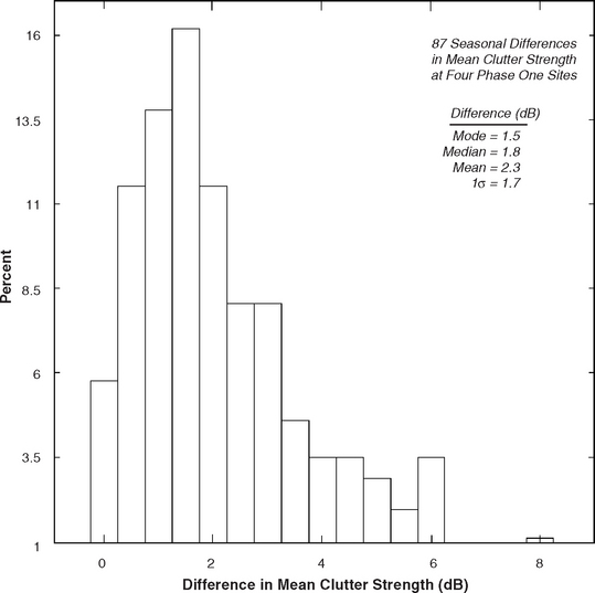
FIGURE 3.48 Histogram of seasonal differences in mean ground clutter strength. Phase One repeat sector data. All five radar frequencies, both polarizations, and both pulse lengths. Sites are Cochrane, Brazeau, and Gull Lake West, two seasonal visits each; and Beiseker, four seasonal visits.
The results of Figure 3.48 for seasonal variation of mean clutter strength indicate that the most likely seasonal variation in mean clutter strength in the Phase One repeat sector measurements (i.e., the mode of the distribution) is 1.5 dB, the average variation is ≈2 dB (i.e., median difference = 1.8 dB, mean difference = 2.3 dB), and the one-sigma range of variability beyond the mean is to 4.1 dB (i.e., 84% of the seasonal differences ≤ 4.1 dB). This value of 4.1 dB is considerably larger than the corresponding value of 2.5 dB in the day-to-day variations, as would be expected. Even so, seasonal changes remain small compared with the total range of variation of mean clutter strength shown in Figure 3.38. The maximum observed seasonal difference in Figure 3.48 is 8.1 dB from Gull Lake West. The maximum seasonal difference at Beiseker is 7.1 dB. For Beiseker alone, the seasonal differences across four visits are just slightly less than the corresponding differences in the four-site data of Figure 3.48. This indicates that seasonal variation is not too different from one site to another.
3.7.3 TEMPORAL AND SPATIAL VARIATION
Figure 3.49 shows cumulative distributions of both diurnal and seasonal variations in mean clutter strength as measured by the Phase One radar. These data come from the histograms of Figures 3.47 and 3.48, respectively. Thus, the diurnal variations shown in Figure 3.49 are based on repeat sector measurements over the two- to three-week stay at every Phase One site. In Figure 3.48, 71% of diurnal variations, largely due to changes in weather, are less than 1.5 dB. The seasonal variations shown in Figure 3.48 are based on six repeated visits by the Phase One equipment to four sites for the purpose of investigating seasonal variability. In Figure 3.49, 71% of seasonal variations are less than 3 dB.

FIGURE 3.49 Diurnal and seasonal variability in mean ground clutter strength. Phase One repeat sector data. All five radar frequencies, both polarizations, and both pulse lengths. Cumulative distributions of data histogrammed in Figures 3.47 and 3.48.
In the foregoing discussion (i.e., Figures 3.47, 3.48, and 3.49), diurnal and seasonal variability in mean clutter strength over repeat sectors are characterized by forming single-sided distributions of absolute values of differences between measurements. This is the natural thing to do when there are only two in the cluster of repeated measurements, for example, two seasonal repeats. When there are more than two in the cluster (e.g., four seasonal repeats at Beiseker), this approach provides all combinations of differences (e.g., six differences among the four Beiseker repeats, although only four were allowed) including the large difference between the two outliers.
The resultant one-sided histogram of absolute values of differences is primarily characterized by the mean, median, and mode of the distribution. In particular, the standard deviation in this one-sided distribution is a secondary or relative attribute that gives the range of variation about the mean difference but, unless quoted with the mean difference, by itself does not provide any absolute information on typically occurring diurnal or seasonal differences. These one-sided histograms are a very satisfactory way to show diurnal and seasonal differences. Even though the number of samples in them grows combinatorially with number of repeated measurements in the cluster (although restricted in the seasonal differences at Beiseker), they do include the difference between each measurement and every other measurement in the cluster (i.e., equal weight to every pair).
Diurnal and seasonal variability in mean clutter strength over repeat sectors may also be characterized, not by forming single-sided distributions of absolute values of differences between measurements, but by forming two-sided distributions of differences of individual measurements from central values within groups of measurements of common frequency, polarization, and resolution. These two-sided distributions of differences from central values provide one-sigma ranges of variability that may be compared with the one-sigma numbers used to specify spatial variability. That is, in considering spatial variation, the distribution of mean strengths is formed from all repeat sector patches of a given terrain class, a central value is determined in the distribution, and variability in the distribution is characterized by the one-sigma range of variation about the central value. To follow a parallel approach for temporal (i.e., diurnal or seasonal) variation, where there are clusters of repeated measurements of each repeat sector patch, it is first necessary to normalize the central value of each cluster to zero to remove patch-to-patch spatial variation. Thus, for each repeated cluster, the central value in the cluster is first specified, then the differences (both positive and negative) of each measurement in the cluster from the central value are determined, and finally all such temporal differences from all clusters are accrued into one aggregate histogram. The resultant histogram of differences is two-sided, approximately symmetric, and approximately normal (i.e., law of large numbers). To repeat, it is showing differences from central values of clusters of repeated measurements, not differences between pairs of measurements in the cluster. It is a two-sided or polarized distribution centered at (or very near) zero. The mean, median, and mode in this two-sided distribution are all at (or very near) zero. This two-sided distribution is primarily characterized by the standard deviation or one-sigma value of the distribution. To the extent that the distribution is normal, 68% of the diurnal or seasonal differences lie within the one-sigma range of variation.
Such two-sided distributions are now provided for diurnal, seasonal, and patch-to-patch variations in repeat sector clutter patch mean clutter strength, respectively. Diurnal and seasonal variations constitute long-term temporal variations for a given patch. Patch-to-patch variations constitute spatial variations from one patch to another within a given category of terrain classification and for a given radar frequency band. These three distributions of variability in mean ground clutter strength are shown in Figure 3.50. In each case, the variation is the difference in mean clutter strength from a central value within a group of measurements repeated in time (i.e., diurnal or seasonal) or in space (patch to patch, for a specific terrain class). Because these data are all similarly derived to show central differences, the three distributions of Figure 3.50 showing diurnal, seasonal, and spatial variability are all primarily characterized by their one-sigma ranges of variability. As is indicated in Figure 3.50, these one-sigma ranges of variability for diurnal, seasonal, and patch-to-patch variations are 1.1, 1.6, and 3.2 dB, respectively.
When all is said and done, the same set of diurnal and seasonal repeat sector measurements exist whether one-sided or two-sided distributions of differences are formed. Thus, aside from statistical niceties, similar numbers should be obtained to characterize typically occurring diurnal and seasonal variations in distributions. To observe the extent to which this is so, consider that the ±1.1 dB and ±1.6 dB one-sigma numbers from the two-sided diurnal and seasonal distributions, respectively, as shown in Figure 3.50, which encompass 79% and 65% of central difference variations, respectively, when doubled to represent absolute differences between individual measurements encompass 80% and 71% of variations, respectively, in the one-sided distributions shown in Figure 3.49.
Each distribution in Figure 3.50 will be discussed in turn. First, the seasonal variations in Figure 3.49 are based on differences in the subset of centrally selected (best) measurements among the day-to-day repeats for the four seasonally revisited sites. The approximate linearity of this curve indicates that the decibel values of seasonal central differences are approximately normally distributed. To the extent that they are, 68% and 95% of them are within one-sigma (i.e., ±1.6 dB) and two-sigma (i.e., ±3.2 dB) ranges of variation, respectively. These percentages are closely approximated by the actual percentages of differences within these ranges of variation, which may be obtained directly from the ordinate in Figure 3.49, as 65% and 94.5%, respectively.
Next, the diurnal variations in Figure 3.50 are based on all repeated experiments at each site, not just the best experiments. In establishing these diurnal variations, experiments with parametric variations that would not be appropriate to attribute to day-to-day variability were eliminated, as were obviously bad experiments due to equipment malfunction. The resultant distribution of diurnal central differences is seen to be approximately normal over its central 60% (from 0.2–0.8 cumulative probability). However, the spreads in the tails (approximately 0–20% cumulative probability on the left side; approximately 80–100% cumulative probability on the right side) of this distribution are considerably greater than would be provided by linear extrapolation of the central quasi-normal distribution. It is apparent in Figure 3.50 that, in the extreme tails (i.e., 1% or 2% on each side), the diurnal differences approach and nearly coincide with the seasonal differences. That is, whatever the mechanisms at work that cause the largest (although infrequent) seasonal changes, mechanisms are also at work to cause similarly large (but infrequent) changes on a day-to-day or weekly basis.
Finally, as were the seasonal variations, the patch-to-patch variations in Figure 3.50 are based upon the subset of centrally selected (best) measurements among the day-to-day repeats. These variations are the differences from the central values given in Table 3.6 of the cluster of measurements in each frequency band in the 12 scatter plots showing mean clutter strength vs frequency by terrain class presented in Section 3.4. In other words, this distribution characterizes the prediction accuracy that may be associated with the generalized values of mean clutter strength by frequency band and terrain type as given in Table 3.6. As with the seasonal variations, the distribution of patch-to-patch decibel central differences in Figure 3.50 is approximately normal over its complete range (i.e., 72% and 94% of differences lie within one-sigma and two-sigma ranges, respectively, compared with 68% and 95% for the normal distribution). However, as would be expected, the distribution of central differences is considerably broader than the distributions of diurnal and seasonal variations (i.e., the one-sigma and two-sigma ranges for patch-to-patch differences are ±3.2 dB and ±6.4 dB, respectively).
The temporal and spatial variability of clutter as given by the distributions of Figure 3.50 is the variability that remains after the data have been separated by terrain type. It is interesting to compare this residual variability with the overall range of variability in the clutter phenomenon without distinguishing terrain type, for example, as is illustrated in Figure 3.39. It is the 3.2-dB one-sigma patch-to-patch spatial variability that determines prediction accuracy based upon repeat sector measurements. The one-sigma patch-to-patch spatial variability in mean ground clutter strength by frequency band before terrain classification is as follows: 16.6, 13.6, 9.7, 7.1, and 5.8 dB, at VHF, UHF, L-, S-, and X-band, respectively (see Table 3.7). In contrast, the corresponding one-sigma patch-to-patch spatial variability in mean clutter strength by frequency band after terrain classification is: 3.9, 3.8, 2.9, 2.7, and 2.3 dB at VHF, UHF, L-, S-, and X-band, respectively. These latter five numbers indicate how the overall 3.2-dB one-sigma spatial variability in Figure 3.50 splits up by frequency band.
In comparing these measures of patch-to-patch spatial variability in mean clutter strength before and after terrain classification, the following observations are made:
• Terrain classification substantially reduces variability in all bands
• The amount of the reduction is greatest at VHF and decreases with increasing radar frequency (i.e., amount of reduction = 12.7, 9.8, 6.8, 4.4, and 3.5 dB at VHF, UHF, L-, S-, and X-bands, respectively)
• The variability after terrain classification still decreases somewhat with increasing radar frequency from 3.9 dB at VHF to 2.3 dB at X-band, but this decrease is very much less than the corresponding decrease before terrain classification
Thus, it is clear that specifying terrain type, terrain relief, and the depression angle at which the terrain is illuminated, as is done in Chapter 3, greatly improves the accuracy to which the mean clutter strength from terrain can be predicted, and that non-terrain-specific approaches to clutter modeling must inherently involve large uncertainties.
3.8 SUMMARY
How strong is radar land clutter? How does the strength of the clutter vary with the type of terrain in which the radar is situated? In particular, whatever the terrain, how does the strength of the clutter vary with radar carrier frequency over the range of frequencies used in modern surface radar operations? These questions have perplexed radar engineers since the advent of radar during World War II. Answers to these questions are important because the performance of surface-sited radar against low-flying targets is often limited by land clutter interference even when state-of-the-art MTI clutter cancellation processing is employed. Because of this importance, many specific clutter measurements have been performed and reported over the years, but they have not led to a characterization of clutter providing generally accepted answers to the above questions.
Central to the difficulty in clutter characterization and prediction is the fact that terrain is essentially infinitely variable, and every clutter measurement scenario is different. Hence, ground clutter’s most salient attribute is variability. As a result, questions concerning clutter strength need to be answered statistically. As is amply illustrated by discussions of individual measurements in Chapter 3, the underlying physics in any given measurement can usually be understood. However, every measurement is fraught with terrain and propagation specifics, and generalization on the basis of any one measurement is usually not possible. The clutter literature, seemingly characterized by inconsistency and contradiction, is really just reflecting the fact that clutter is an extremely variable statistical process. The literature frustrates us with single-point measurements of which the broader significance is not understood.
Thus, a major new program of ground clutter measurements was undertaken at Lincoln Laboratory to provide new general understandings and predictability of the low-angle ground clutter statistical phenomenon. Large amounts of data were collected in the belief that averaging over large amounts of data would allow underlying fundamental trends to emerge that are often obscured by specific effects in individual measurements. The five-frequency Phase One clutter measurement radar system was operated continuously in the field over a three-year period, collecting multifrequency clutter data at 42 different sites.
Many of the measurement sites were in western Canada, in terrain of relatively low-relief and at northern latitudes. In addition to this emphasis, however, many other important terrain types were measured, including mountains, cities, desert, marshland, farmland, and woodland. Many of the Phase One sites and the measurements obtained there are described in Chapter 3. Altogether in this measurement program, approximately 475 gigabytes of accurately calibrated, pulse-by-pulse ground clutter data were collected.
Chapter 3 provides multifrequency results of low-angle clutter based on the repeat sector database which altogether comprises 4,465 clutter measurements. The repeat sector at each site was an azimuth sector of concentration in which measurements were repeated a number of times to increase the reliability of the results. As an easy-to-comprehend summary, Figure 3.38 and Table 3.6 represent the best repeat-sector answers to the most pressing high-level questions for which answers were sought in the Phase One clutter measurement program.
The results of Figure 3.38 and Table 3.6 have a number of advantages. First, underlying them is a universally applicable terrain classification system consistently applied across 42 different repeat sectors. This classification system causes the clutter statistics to cluster within class and to properly separate between classes. This system separates differences in terrain or measurement scenario that are enough to cause significant variation (i.e., different classes) in the clutter returns. The terrain classification system utilized is basically formulated at 1:50,000 scale to classify both land-surface form and land cover, and quantifies important parameters such as terrain relief, terrain slope, depression angle, and percent tree cover.
Second, the data shown in Figure 3.38 and Table 3.6 are medianized and hence generalized central values within terrain classes. Even at best, terrain is variable within class, and any single measurement in a given terrain class comes from a spectrum of all possible measurements in such terrain. The data shown in Figure 3.38 and Table 3.6 are medianized central values over many measurements and thus represent generally occurring levels of clutter strength in each terrain class. Third, the data of Figure 3.38 and Table 3.6 were accurately calibrated and reduced using consistent data reduction procedures. Complicating factors in data reduction, such as electromagnetic propagation (ground clutter is not a free-space measurement), geometric shadowing (a dominant influence in the low-angle regime), radar sensitivity limitation, radar noise contamination, and differing degrees of coherency in clutter returns are explained in Chapter 3. Finally, each measurement underlying the medianized data of Figure 3.38 and Table 3.6 is itself a centrally selected measurement from a group of identically repeated measurements in which occasional anomalous outliers have been removed. Thus, the summary results of Figure 3.38 and Table 3.6 are the product of much effort devoted to concerns with accuracy, generality, and statistical consistency.
The results of Figure 3.38 and Table 3.6 are now summarized. First, these results indicate 66 dB of variability in mean strength of ground clutter from mountains at VHF to marshland or desert at UHF. However, these results also provide a rational means of sorting through this variability, through specification of terrain type, relief, depression angle, and radar frequency. In general terms, it is seen that just five major, easy-to-distinguish terrain categories are utilized; namely, mountains, cities, forest, farmland, and, as an encompassing fifth category, desert, marsh, or grassland with few large discrete clutter sources. As expected, mountains and cities produce strong clutter returns, and desert, marsh, and grassland produce weak clutter returns. Results from the preceding Phase Zero X-band program of ground clutter measurements described in Chapter 2 show that, at the very low angles of ground-based radar, depression angle as it affects shadowing on a sea of discrete clutter sources is of dominant importance to clutter statistics. The Phase Zero findings are essentially duplicated in the Phase One X-band results of Figure 3.38 and Table 3.6. In addition, similar important dependencies on depression angle at the other frequencies, VHF, UHF, L-, and S-bands, are observed, such that fractional variations of depression angle cause major variations in clutter statistics in all these bands.
However, the purpose of Chapter 3 is not so much to dwell on the previously emphasized important role of depression angle, which also fundamentally affects statistical spreads in distributions, but to take up the question of frequency dependence in these distributions. The question of frequency dependence requires an empirical approach. The summary data of Figure 3.38 and Table 3.6 show that in forest of high relief and/or at high depression angle, mean ground clutter strengths decrease significantly with increasing frequency; whereas, in very low-relief farmland, mean ground clutter strengths increase significantly with increasing frequency. The frequency dependence of mountain clutter mirrors the behavior of high-relief forest clutter, except that it is stronger; the frequency dependence of desert or marshland clutter mirrors that of very low-relief farmland, except that it is weaker. (An exception occurs where, at high depression angle at X-band, desert clutter is as strong as forest clutter.) For much commonly occurring terrain, either farmland or forest of moderately low-relief leading to intermediate illumination angles, little general dependence of mean clutter strength with frequency is observed. In such terrain, mean clutter strengths hover around the −30-dB level, VHF to X-band. In summary, the data of Figure 3.38 and Table 3.6 bring much statistical order to the problem of predicting mean clutter strengths from spatial macroregions of terrain. They answer the questions of how strong clutter is for various terrain types and for radar frequencies varying from VHF to X-band. These numbers are subsequently refined in the clutter modeling information presented in Chapter 5.
Within any spatial macroregion consisting of hundreds or thousands of resolution cells, extreme cell-to-cell fluctuation occurs about the mean value as provided by Figure 3.38 and Table 3.6. A proper clutter model will model these statistical fluctuations. The clutter models subsequently developed in Chapters 4 and 5 do so by modeling the clutter returns as random numbers from Weibull distributions. Each modeled Weibull distribution is characterized by a mean strength and a shape parameter. Any model needs to reach towards simplicity and generality. Thus, in the clutter model of Chapter 4, some subjective smoothing of trends is performed as complementary results from the Phase Zero and Phase One programs are merged and minor variations that are judged to be statistically insignificant are removed. The results of Figure 3.38 and Table 3.6 are exact results as delivered by the repeat sector measurements, medianized within terrain class and including both vertical and horizontal polarizations and high and low range resolutions.
Chapter 3 provides general information on the effects of polarization, range resolution, weather, and season on mean clutter strength. The effects of each of these parameters are generally small, primarily because mean clutter strength is dominated by strong discrete clutter sources that are physically complex with respect to polarization and relatively invariant with weather and season. With polarization, only a slight overall trend exists where vertical polarization provides stronger mean clutter than horizontal by 1.4 dB on the average. However, the one-sigma variability about this average is 2.8 dB, and occasional differences in mean strength with polarization can occur in the 5- to 10-dB range, with either vertical or horizontal being stronger. Radar resolution fundamentally affects spreads in clutter amplitude distributions, not the means which are emphasized in Chapter 3. Across all the repeat sector measurements, the mean strength measured at high resolution is only 0.8 dB stronger on the average than that measured at low resolution. The one-sigma variability with resolution about this average is 2.2 dB. Variations of mean strength with resolution indicate the existence of small numbers of discrete interfering scatterers within a resolution cell.
Weather and season act to introduce statistical variability in mean clutter strength without apparent trend. On the basis of the repeated measurements at each site, the one-sigma variability due to short-term changes with weather is specified at 1.1 dB, with occasional variations (i.e., 10%) greater than 3 dB. On the basis of the seasonal revisits to six sites, the one-sigma variability due to long-term changes with season is specified at 1.6 dB with occasional variations (i.e., 10%) greater than 4.8 dB. These specifications of diurnal and seasonal variability in terms of probability of occurrence bring statistical order to a historical literature characterized more by individual examples. The long-term diurnal and seasonal temporal variabilities of mean strength in the repeat sector measurements of 1.1 dB and 1.6 dB, respectively, may be contrasted with the sector-to-sector spatial variability within groups of common terrain type in the measurements. This spatial variability has a one-sigma range of 3.2 dB, which represents a measure of prediction accuracy based on repeat sector measurements. In light of such variability (seasonal, weather related, and spatial), the reader is cautioned that the numbers comprising the clutter modeling information of this book need to be regarded as statistical averages. These averages certainly establish important trends. Any specific clutter measurement, however, whether new or historical, may vary considerably from these predicted average numbers.
Chapter 3 emphasizes mean clutter strengths over spatial macroregions consisting of many contiguous resolution cells. The most basic descriptive measure of any statistical distribution is the mean of the distribution, which is the average of all the samples in the distribution, each sample weighted by just its own strength. The means usually occur high in the measured clutter amplitude distributions, often near the 90-percentile level, driven there by occasional strong returns from discrete sources. However, because the distributions are not simply behaved does not mean that the standard techniques of statistical science for bringing them under general description should be discarded. This seemingly self-evident fact is mentioned here because means at high percentile levels can occasion a sense that they should be discounted. Returns from discrete sources over a wide range of strengths comprise the phenomenon for which a description is sought. The phenomenon is not so simple that, for example, moving to the median can rid it of a few classical, water-tower type of contaminating discretes and thus provide a better central measure of a well-behaved, discrete-free clutter background.
For complete descriptions of the repeat sector clutter amplitude distributions in addition to mean levels, general information is also provided in Chapter 3 on higher moments and percentile levels, medianized over a number of individual repeat sector measurements within the same terrain groups as the means. The higher moments provided are standard deviation, skewness, and kurtosis. The standard deviation is the basic statistical measure of spread, and from it the Weibull shape parameter of the clutter models developed in Chapters 4 and 5 is completely determined. Skewness and kurtosis are normalized third and fourth central moments, respectively. These quantities are of particular importance in theoretical investigations. The percentiles provided in Chapter 3 are the 50-, 70-, and 90-percentile levels in the clutter amplitude distributions. They provide an easy descriptive means of visualizing the distributions, although otherwise they contain less meaningful statistical information in three or four numbers than do the moments.
Chapter 3 provides mean land clutter strength vs radar frequency, VHF through X-band, as measured over repeat sector spatial macroregions of terrain at 42 different sites. These results were obtained under one unified program of measurements utilizing consistent and accurate calibration throughout. As such, they provide much information on the frequency dependence of radar land clutter and in totality bring connecting tissue to a disjointed literature. Many of the results, at least in detail, are specific to the site at which they were obtained. Chapter 3 averages out such specificity by combining results from sites of similar terrain class. In this manner, generalized characteristics of mean land clutter strength vs frequency are arrived at for most important terrain types.
The information in Chapter 3 on the frequency dependence of low-angle land clutter is based on a statistical population of just 42 repeat sector clutter patches. When these 42 samples are divided up among five major categories of terrain and then further partitioned by relief and depression angle, they do not leave very many samples per category. The Phase One multifrequency 360° survey data at each site provide clutter amplitude distributions for many more patches, on the order of 80 patches per site as opposed to the one patch per site provided by the repeat sector database. Results based on survey data are subsequently provided in Chapter 5, substantially improving the statistical rigor with which multifrequency clutter characteristics are specified.
Appendix 3.A PHASE ONE RADAR
3.A.1 Phase one sites
A photograph of the Phase One ground clutter measurement equipment deployed at the Katahdin Hill site at Lincoln Laboratory is shown in Figure 3.A.1. The Phase One measurement program consisted of setting up and acquiring clutter measurement data with this equipment 49 times at 42 different sites. Table 3.A.1 lists the 49 Phase One site visits, and for each provides the site location by latitude and longitude, the time of year of the measurements, the number of sections that were extended in the expandable Phase One antenna tower, and whether the visit was a repeated visit (n) to the site to establish seasonal variations.

3.A.2 PHASE ONE MEASUREMENT EQUIPMENT
Important Phase One system parameters are shown in Table 3.A.2. The five Phase One frequency bands—VHF, UHF, L-, S-, and X-bands—shared three antenna reflectors. The large 10-ft by 30-ft reflector was a shared dual-frequency antenna between VHF and UHF with each band having its own set of crossed dipole feeds. A photograph of this VHF/UHF feed system is shown mounted in position in front of the VHF/UHF reflector in Figure 3.A.2. The intermediate-sized reflector was a similar shared reflector between L- and S-bands, with a crossed dipole feed at L-band and a dual polarized waveguide feed at S-band. The L- and S-band feeds were protected by a radome. A smaller reflector was dedicated to X-band, which was fed with a dual-polarized horn. A close-up view of the L-/S-band radome and the X-band reflector above it is shown in Figure 3.A.3. Visible above the X-band reflector in this photograph is a TV camera that provided a boresight video display at the operating console in the electronics trailer.


The antenna tower upon which the three reflectors were mounted was expandable in six sections to a nominal maximum height of 100 ft. The weight on top of this tower due to the five antenna systems and associated equipment was 3,000 lbs. The antenna wind load was 8,000 lbs at the specified survival wind velocity of 75 knots. The tower was guyed with 28 cables, each tensioned to 1,000 or 2,000 lbs. Eight guy anchors were emplaced at each site and each was tested to 20,000 lbs withholding capacity. Motion at the center of mass on top of the tower, critical to system stability and phase coherence, was tested to within a specified tolerance (viz., 0.1035 in/sec) under dynamic wind loading using a vertically directed laser.
Table 3.A.2 shows gains, beamwidths, and rms sidelobe levels of the Phase One antenna beams at a particular selected frequency within each band. The Phase One system was capable of operating within a 5% bandwidth in each of its five radar bands. The frequencies shown in Table 3.A.2 were those most commonly used in Phase One data acquisition. The antenna beams were relatively wide in elevation and were fixed with boresight horizontal at 0° depression angle (i.e., no control was provided on the position of the elevation beam).
The azimuth and elevation beamwidths specified are as measured at the 3-dB one-way points (6-dB two-way). For most sites and landscapes, the terrain at all ranges from 1 to many kilometers was usually illuminated within the 3-dB points of the fixed elevation beamwidth. The measured clutter statistics are corrected for gain variations on the elevation beam both within and beyond the 3-dB points, depending on the off-boresight angle to the backscattering terrain point. At almost all sites, either three antenna tower sections were raised to provide a nominal height of 60 ft or six tower sections were raised to provide a nominal height of 100 ft. Occasionally, some clutter data were acquired with only one or two tower sections raised to provide nominal heights of 30 ft or 45 ft, respectively. The number of tower sections used at each site is shown in Table 3.A.1.
The Phase One equipment constituted a self-contained transportable five-frequency radar system transported by three tractor/trailers (see Figure 3.A.1). The white electronics trailer contained the five transmitters, receivers, exciter, analog-to-digital (A/D) converters, signal processors, a digital computer, displays, and high-speed data recorders. The flat-bed tower trailer transported the tower, antenna reflector midsections, antenna feeds, and a diesel-operated winch system used to erect the tower. The tarpaulin-covered equipment trailer transported a 60-kW diesel generator, waveguide sections, coaxial RF cables, power cables, a man-portable 75-ft tower used during system calibration, and portions of the antenna reflectors.
The overall radar system block diagram is shown in Figure 3.A.4. The system exciter supplied all transmit and receive local oscillator (LO) frequencies and provided the basic timing reference for the system. The basic frequency reference for the exciter was a Hewlett Packard 8662A synthesizer signal generator, which had sufficient stability to support an overall system clutter improvement factor of 60 dB. There were five transmitters in the system. The two higher frequency transmitters (S- and X-bands) had traveling wave tubes (TWTs) as final high-power output stages. The intermediate and final stages of the three low band transmitters (VHF, UHF, and L-band) used Eimac type Y-739F planar triodes with Eimac CV-8030 series resonant cavities. A single low-band transmitter power supply was used for intermediate and final stages of the three low-band transmitters. The cavities could be manually tuned over a few megahertz in each of the three low-band transmitters. The signals from each of the five high-power transmitters were fed through their respective circulators to transmission lines. The S- and X-band signals were transmitted to their antennas in separate waveguides. The two waveguide runs consisted of 12-ft sections connected together during tower erection. A single 7/8-inch coaxial line was used to carry the VHF, UHF, and L-band signals to their antennas. The appropriate low band signal was switched into the coaxial line by two three-way band-select switches, one located near the top of the tower, and the other inside the electronics van. The signal received from each antenna was fed to a separate preamplifier for each frequency band. The first intermediate frequency (IF) for all frequency bands was 740 MHz. The first IF entered into a common receiver used for all frequencies.

The diagram of the receiver and signal processor is shown in Figure 3.A.5. The receiver IF gain could be varied dynamically according to an r3 or r4 (where r = range) sensitivity time control (STC) function. Both STC functions provided 40-dB attenuation at 1 km. In addition, the preamplifiers shown in Figure 3.A.4 could be bypassed, and fixed attenuation could be switched into the system to avoid system saturation by large target returns. The 740-MHz IF signal was mixed to 150 MHz where the matched filtering was accomplished. Additional IF amplification was also provided. The 150-MHz IF signal was converted to in-phase and quadrature (I and Q) signals at baseband where the A/D conversion was performed.

The Data Collection Unit provided real-time buffering of the I and Q data and routed the clutter data to the PDP-11 computer or tape recorder. The Radar Data Processor (RDP) performed envelope detection, or the I and Q samples were fed to a digital-to-analog (D/A) converter which drove the A-scope as shown. In addition, the RDP performed real-time noncoherent integration of 128 pulse returns. The integrated data were saved by the computer, which, in non-real time could generate a range/azimuth display. The Radar Control Unit consisted of timing and data control logic that accepted commands from the computer and converted them to radar control signals. Data collection was controlled automatically by the computer. The system operator input parameters via keyboard or floppy disk which established the range and azimuth limits, radar frequency, scan rate, waveform, sampling rate, and polarization to be used for each experiment (see Table 3.A.8).
TABLE 3.A.8
Radar Directive File Parameters for Clutter Data Collection Experiments
| Measurement Sector | Radar Parameters |
| Range (km): (a) START (b) EXTENT | Frequency: VHF, UHF, L-, S-, X-Band |
| Azimuth (deg) (a) START (b) STOP | Polarization: VV or HH |
| Antenna Mode | Resolution (m): 15, 36, 150 |
| (1) Step: (a) Azimuth increment (deg) | Range Sampling |
| (b) Number of recorded pulses < 30,720 | Rate (MHz): 1, 2, 5, 10 |
| or | PRF (Hz): 500, 1000, 1500, … 4000 |
| Record 1 out | |
| (2) Scan: (a) Scan velocity ≤ 3 deg/s | of N Pulses: N = 1, 2, 4, 8, 16 |
| Attenuation: | |
| Fixed: 1, 2, 3, … 40 dB | |
| STC: r3 or r4; 40 dB at 1 km |
The Phase One system performance parameters listed in Table 3.A.2 are now described more fully. System stability and dynamic range are commensurate with a clutter improvement factor of 60 dB at VHF, UHF, and L-band and 55 dB at S- and X-bands for a two-pulse cancellation technique. These specified clutter improvement factor levels assume that pulse-to-pulse variations in transmitter amplitude and phase due to antenna motion are small. The pulse-to-pulse variations in transmitter amplitude and phase were measured in real time and stored on tape in the calibration block of the clutter data record. Experimental tests showed that antenna motion was minimal and that 60-dB clutter improvement performance was achieved in winds up to 20 knots. The Phase One system was capable of transmitting and receiving vertical or horizontal polarization.
There were two waveforms available at each frequency, one at low resolution (150 m) and one at high resolution (15 m at L-, S-, and X-bands; 36 m at VHF and UHF). The waveforms were short uncoded pulses of 1-μs duration for low resolution and of 0.1-μs or 0.25-μs duration for high resolution. The minimum range of 1 km is the closest range from the radar at which clutter data could be collected. The calibration accuracy specification of 2-dB rms reflects the capability of maintaining this accuracy across all sites (see Section 3.A.3). The instantaneous dynamic range was the amplitude range of clutter strength that could be collected with a signal-to-noise (S/N) ratio of 12 dB or greater without saturating or exceeding the linear range of the receiver and A/D converter. The center of the 60-dB instantaneous range could be adjusted in 1-dB steps from 0 to 40 dB. For example, the total dynamic range could be expanded to 100 dB by first collecting data with 40 dB of attenuation over a particular area and then repeating the data collection over the same area with no attenuation. Additional control of dynamic range could be effected through bypassing the preamp.
The clutter data were recorded in I and Q format at the A/D converter outputs. The maximum A/D converter sampling rate was 107 I and Q samples per second with 13 bits each. The A/D data were then buffered for the recorders, which had a maximum recording rate of ≈625 Kbytes per second. The system sensitivities shown in Table 3.A.2 apply to the 150-m waveform. The sensitivity to clutter for the high resolution waveforms was 20 dB lower (10 dB reduction in pulse energy, and 10 dB reduction in area illuminated).
There were three basic data collection modes available: the beam scan mode, the parked beam mode, and the beam step mode. During the beam scan mode, data were collected as the antenna beam scanned from one azimuth limit to the next. In the parked beam mode, data were collected while the beam was held at a fixed azimuth—long-time-dwell data were collected with a parked beam. In the beam step mode, the beam was stepped through the measurement sector, beam position by beam position, with the beam held fixed at each step while data were recorded. Approximately 15 s were required for antenna stabilization at each step during step beam data collection. Largely because of this antenna stabilization wait time in step mode, most of the 360° survey data were recorded in scan mode to keep data volume and data acquisition time reasonable. However, many of the repeat sector measurements were conducted in step mode. See Section 3.C.4 for computational comparison of clutter measured in these various modes. The antenna scan was limited to 360° due to cable wrap.
3.A.3 PHASE ONE CALIBRATION
Each operating mode of the Phase One radar had an adjustable system range bias associated with it. These range biases were accurately adjusted when the equipment was first set up at Katahdin Hill at Lincoln Laboratory. These initial adjustments were made by measuring radar reflections from known discrete targets in the neighborhood for which the positions had been accurately surveyed. Range calibration was checked at every Phase One site in a boresight test using a prominent discrete object of opportunity (such as a water tower) as a radar target, the radar range of which was obtained from large-scale maps.
Azimuth information was provided in the Phase One system by a precision azimuth encoder in the servo drive mechanism for steering the antennas. Every recorded pulse had associated with it in header information an azimuth position read from this encoder. The quantization interval of the encoder was 0.01°. Occasionally, even with a fixed beam position, wind forces could cause very small positional variations which, even though small, were picked up by the encoder and precisely recorded on tape. The raw azimuth-encoded data indicated relative angle information only and had to be corrected by an additive offset to provide absolute azimuth with respect to true north. The correction angle varied from site to site, depending on the particular setup geometry realized by the trailer configuration at each site. The same boresight test that checked range calibration at each site using a prominent discrete target also was used to provide the azimuth servo correction angle.
Phase One signal strength calibration involved both internal and external procedures. Every recorded clutter experiment carried with it on the raw data tape both pre- and post-calibration files containing internally measured values of transmitter and receiver parameters. Table 3.A.3 lists the parameters that were internally measured and recorded with each experiment and indicates the frequency at which these measurements were performed. These parameters were subsequently used at Lincoln Laboratory to reduce the data to units of absolute clutter strength on calibrated clutter tapes. The automatic internal calibration measurements shown in Table 3.A.3 calibrated the Phase One system up to the transmit and receive couplers. Beyond these couplers, the RF transmission line losses and antenna gains were checked by external tests. Table 3.A.4 summarizes these external tests, which include range and azimuth calibration as discussed above.
TABLE 3.A.3
| Test | Frequency |
| Receiver gain | Each experiment |
| Transmitter average power | Each experiment |
| Transmit amplitude and phase | Each pulse |
| Antenna VSWR | Operator request |
| Receiver noise figure | Half hour |
| Synchronous detector balance | Half hour |
| DC correction loop | Half hour |
| Fixed attenuator | Each experiment |
| Sensitivity Time Control (STC) | Each experiment |
TABLE 3.A.4
| Test | Frequency Bands | Purpose |
| Standard gain antenna tests (receive and transmit) | VHF, UHF, L-Band | Signal strength calibration |
| Corner reflector tests | S-Band, X-Band | Signal strength calibration |
| Boresighting tests | All bands | Range and azimuth calibration |
| Reference object tests | All bands | Signal strength monitoring |
External signal strength calibration checks were conducted using standard gain antennas and corner reflectors. The standard gain antenna tests were conducted as both receive tests and transmit tests at VHF, UHF, and L-band; corner reflector tests were conducted at S-band and X-band. The lower band receive tests consisted of radiating a signal from a standard gain antenna (horn at L-band, Yagis at VHF and UHF) located on a tower approximately 100 m from the radar tower, and receiving this radiated signal at the Phase One receiver. In these procedures, the standard gain antenna was located on the fringe of the near field of each of the three low band Phase One radar antennas. A Hewlett Packard 866A signal generator was used for the RF source. The RF signal was transmitted through a 100-ft coaxial cable to the standard gain antenna on top of the calibration tower which could be expanded from 37 to 75 ft. By raising and lowering the tower, the multipath effects were accounted for by measuring the maximum and minimum signal level and calculating the free-space signal assuming a relatively constant terrain reflection coefficient. At the 100-ft radar tower height the multipath was usually less than 2 dB at all of the low band frequencies. At the 60-ft radar tower height the multipath effects remained small at UHF and L-band but were somewhat more significant at VHF. The lower band transmit tests were conducted by transmitting from the Phase One radar and receiving at the standard gain antenna. The equipment and procedures were identical to the receive tests except that a Hewlett Packard 1/36A power meter was used to measure the power received at the standard gain antenna.
The external calibration tests at S- and X-band were conducted using a corner reflector for which the RCS was +35.7 dBsm (i.e., dB with respect to 1 m2) at X-band and +27.5 dBsm at S-band. The corner reflector was mounted on the calibration tower approximately 3 km from the radar tower and was raised and lowered to account for multipath reflections similarly to the transmit and receive standard gain antenna tests. Where possible a line of brush or small trees was used to block the terrain multipath. The X-band returns seldom varied by more than 2 dB, but the S-band returns more frequently varied by more than 2 dB. Measurements of the calibration tower without the corner reflector indicated that the tower RCS was approximately 10 dB lower than the corner reflector RCS at S-band.
Calibration constants were not individually adjusted at each site on the basis of each site’s external calibration tests because the calibration tests were always conducted in a nonfree-space propagation environment and hence had some associated site-specific variation. Instead, average results over a multisite history of external tests were used to set calibration constants. This leaves site-to-site variations over the history of the external tests. Table 3.A.5 shows the standard deviation by band and polarization in the site-to-site variations in the Phase One external calibration measurements over the history of the program. Table 3.A.6 shows similar data from a single reference target for the Phase One radar’s subsequent nine-month setup on Katahdin Hill. As expected, the variations occurring at a fixed site (Table 3.A.6) are less than those occurring across many sites (Table 3.A.5). The variations shown in both Tables 3.A.5 and 3.A.6 are small and validate the quoted estimate for calibration accuracy of ≈2 dB rms across the complete set of Phase One sites.
TABLE 3.A.5
Standard Deviations (dB) of External Calibration Measurements over the Three-Year History of the Phase One Radar*

*External calibrations were performed at 36 Phase One sites using a corner reflector and standard gain antennas. The standard deviations are of differences between expected and measured results. Calibration constants were set such that mean values of these differences over multiple sites were zero.
TABLE 3.A.6
Standard Deviations (dB) of Measurements of Reference Target RCS at Katahdin Hill over Nine-Month Period*

*The Phase One radar collected ground clutter and reference target data once a week over a nine-month period at the Katahdin Hill site. The referenced target was a 120-ft tall, 40-ft diameter cylindrical water tank located at a range of 6.5 km.
†Severe VHF interference frequently occurred at the Katahdin Hill site, which may have affected the consistency of the VHF measurements.
At each site, the discrete reflecting object such as a water tower used in boresight range and angle calibration was also used as a signal strength reference target prior to and throughout clutter data collection (see Table 3.A.4). The return from the reference object was repeatedly measured and recorded to ensure that no changes occurred in system calibration. As a result, a set of measurements of reference target RCS in each band was available from each site. For each site and band, the standard deviation across this set of measurements was computed. Table 3.A.7 shows the mean values of these standard deviation numbers in each band across all sites. The data in Table 3.A.7, which summarize many more measurements than Tables 3.A.5 and 3.A.6, confirm day-to-day calibration repeatability based on measurements from reference objects such as water towers.
TABLE 3.A.7
Standard Deviations (dB) of Measurements of Reference Target RCS at 33 Sites*

*Daily reference target data were collected at 33 Phase One sites over the radar’s three-year history. At each of these sites, a strong discrete reference target of opportunity, such as a nearby water tower, was selected to check day-to-day system repeatability.
3.A.4 PHASE ONE DATA COLLECTION
The basic entity in which Phase One data were recorded was as a Clutter Data Collection (CDC) experiment. In each experiment, clutter returns were measured pulse by pulse from every resolution cell on the ground over some area defined by beginning and ending limits on both range and azimuth for a given antenna mode and for a fixed set of radar parameters. Each experiment was defined by a Radar Directive File (RDF). The RDF controlled the Phase One measurement system during acquisition of the clutter data within each experiment. The RDF parameters requiring specification for each CDC experiment are shown in Table 3.A.8. The measured clutter data were obtained as either survey, repeat, or long-time-dwell data.
Appendix 3.B MULTIPATH PROPAGATION
3.B.1 BACKGROUND
In considering the physics of the low-angle clutter phenomenon, an important factor is the effect of the intervening terrain on the illumination at the backscattering cell. As is indicated in Figure 3.B.1, the terrain between the radar and the clutter patch influences the illumination of the clutter patch. For example, multipath reflections can interfere with the direct illumination and cause lobing on the free-space antenna pattern. All terrain propagation effects including reflection and diffraction are included within the pattern propagation factor F (see Section 2.3.1.2). Ideally, one would wish to separate effects of propagation from the backscatter measurement.

However, the actual effects of terrain on illumination cannot be easily separated out. To do so experimentally would require a separate measurement of illumination strength in every clutter cell. As to what this would entail, consider that the illuminating field strength is often a rapid function of elevation near the ground, making it difficult to determine the actual illuminating field distributions over typical vertical clutter features (e.g., tree, silo). To do so theoretically requires use of radar propagation prediction computer codes, utilizing digitized terrain elevation data, such as those based on SEKE [1, 2], Parabolic Equation [3–5], or Method of Moments [6]. At X-band, such codes are useful for providing physical insight on the statistical average over large spatial regions at clutter source heights, but are not accurate enough to allow deterministic cell-by-cell computation and separation of F in clutter measurement data. At VHF, however, propagation variation exhibits less scintillation and some efforts were made to use propagation prediction codes to predict and separate F from Phase One VHF clutter measurements. However, these attempts to separate F in VHF clutter data generally met with little success because the local cell-to-cell variations in clutter strength σ°F4 were not well correlated with the predictions of F—the resultant separated distributions of intrinsic σ° usually became broader instead of narrower than the corresponding distributions of σ°F4.
Therefore, what is measured as real-world clutter strength is the product of the clutter coefficient, σ°, defined (see Section 2.3.1.1) to be RCS per unit ground area in the resolution cell, and the fourth power of the pattern propagation factor. The propagation factor is raised to the fourth power as it enters into clutter strength because clutter strength (actually clutter intensity) is proportional to power (i.e., the square of the field strength), and a two-way propagation path is involved. Implicit in this definition of clutter strength is the proper assumption of unit plane wave illumination in the definition of RCS, as well as the proper incorporation of the real unknown illumination within the propagation factor. Throughout this book clutter strength is represented by the symbols σ°F4 to demonstrate explicitly that clutter strength depends on two important factors, the intrinsic backscatter and the illumination. These two factors are not separated in the clutter measurement data or clutter results in this book.
Within the Phase One clutter measurement program, measurements of illumination strength and the effects of propagation on illumination were made at a number of Phase One sites. These propagation measurements were recorded in a helicopter (i.e., Phase One radar used as transmitter; receiver in helicopter) flying vertical ascents and descents above selected clutter cells. The important findings from these propagation measurements are incorporated in the interpretation of the clutter measurement data in this book.
At X-band, terrain reflection coefficients are often lower and hence multipath effects are diminished from those that can exist at lower radar frequencies. The Phase One propagation measurements revealed, however, that significant multipath lobing does exist at X-band on typical low-relief open prairie landscapes. When they exist at X-band, propagation lobes are relatively narrow—for example, the height to the first maximum on the X-band lobing pattern is 14.6 ft at 10-km range with a 60-ft antenna tower over a level reflecting surface. Typical clutter sources such as trees and buildings over most visible terrain often subtend a number of such lobes when they exist. As a result, the effects of propagation are further diminished at X-band when compared with lower frequencies.
As carrier frequency decreases, especially below L-band to UHF and VHF, influences of terrain on propagation and illumination strength can become dominant. First, at the lower frequencies, terrain reflection coefficients increase so that multipath lobing becomes stronger. Second, for a given antenna height, as carrier frequency decreases, the widths of the multipath lobes become broader—for example, the height to the first maximum on the VHF lobing pattern is 864 ft at 10-km range with a 60-ft antenna tower over a level reflecting surface. This result may be understood on the basis of the lobing pattern simply being an interference pattern between the actual source of radiation and its image in the reflecting terrain surface. For a given antenna height, as carrier frequency decreases, the effective separation of the source point and its image measured in wavelengths decreases, and the angular periodicity (i.e., lobe width) in the interference pattern increases.
Even at X-band, there can be a region at long enough range where strengths from even relatively high clutter sources are generally reduced because of illumination from the underside of just the first propagation lobe. In contrast to such a relatively unusual X-band situation, however, at lower frequencies these broad multipath lobes can be of dominant influence even at short ranges over typical sources and patches. That is, they can strongly change (either increase or decrease) the effective gain over whole clutter patches and over the complete vertical extents of typical clutter sources within patches. This situation is illustrated in Figure 3.B.1 where a strong low-frequency multipath lobe caused by a terrain reflection coefficient ρ of unity increases effective antenna gain over the whole patch by 12 dB. Such an increase is evident in the Strathcona repeat sector clutter measurements at VHF. The theoretical upper limit to gain increase over free space caused by a single Fresnel multipath reflection is 12 dB, which is the result of both incident and scattered field strengths being doubled by terrain reflection, although terrain focusing effects can occasionally result in gain increases > 12 dB.
The Phase One clutter data are analyzed to determine important fundamental trends in clutter strength σ°F4 as measured from regions of visible terrain. Except at low frequencies on level open terrain, the effects of multipath propagation on clutter strength are usually specific to the particular terrain profile occurring for any given measurement and hence statistically dispersive across a set of nominally similar measurements as the details of the multipath lobing vary from measurement to measurement. Thus, the measurement program requires many sites and patches to overcome such specific influences. As noted, it might be initially supposed that the theoretical high ground would be to separate propagation from backscatter. This becomes even more the case upon considering that illumination strength of a discrete vertical clutter source in the presence of multipath is a function of geometrical factors such as antenna height and range to the clutter source. The practical goal in this book is to move in a statistical fashion past this impracticable position requiring the separation of propagation effects to provide useful results for predicting low-angle ground clutter strengths as actually experienced in ground-based radar. The process involves gathering statistics as much on propagation F as on terrain backscatter σ°.
It is evident from the above discussion that the propagation factor F significantly affects clutter strength σ°F4. It is oversimplifying, however, to attribute most of the variability in σ°F4 over any given spatial macroregion to propagation. The Phase One measured clutter histograms over such macroregions reveal up to 60 dB of cell-to-cell variability in intrinsic σ° over forested terrain where effects of propagation are minimal (i.e., F ≅ 1); this variability increases to 80 dB over open terrain supportive of multipath. Thus the measurements indicate that most of the cell-to-cell variability within patches in the measured clutter data is associated with variations in intrinsic σ°, although variations in propagation F further increase the variability in clutter strength σ°F4. Preliminary attempts [7] to model the low-angle clutter phenomenon as constant σ° with a subsequent overlay of propagation computation were not in the end generally successful in accurately replicating measured clutter amplitude distributions. Of course attempts to model low-angle clutter as constant σ° without including effects of propagation are even more unrealistic—studies have shown that the value of constant σ° (i.e., the percentile level in the measured clutter distribution) that provides equivalent system performance as real clutter is highly specific to the particular system, performance parameter, and terrain being modeled.
The idea of extreme variability in intrinsic clutter σ° is not always intuitive. For example, consider two similar pine trees—how can their intrinsic σ°’s be very different from each other? Hence it must be propagation-induced variations in the illumination of the trees that cause such wide variations in measured clutter strength. However, what is not accounted for in such an argument is that the clutter measurement is made at low angles over a spatial macroregion encompassing a number of square kilometers of forested terrain with all of the cell-to-cell variability that naturally occurs over such terrain including local effects of shadowing where the treetops drop out of visibility and discretes where tall trees rise into visibility. It is true that cell-to-cell variations in illumination within and over a forest canopy are largely propagation induced, but such microscale variations involving inter- and intra-tree propagation effects are properly subsumed within intrinsic σ°, and are not the sort of macroscale propagation effects caused by significant variations in terrain elevation that can realistically be predicted by available propagation prediction codes and included in the propagation factor in the measurement data. Such discussion makes clear the futility of attempting to too finely distinguish effects of propagation from those of intrinsic clutter—at low angles, both clutter and propagation are to a significant degree bound up as one integrated and inseparable phenomenon, as put forward in a theoretical discussion of low-angle scatter by Barrick [8].
The SEKE propagation code [1, 2] was utilized to estimate propagation at clutter source heights in many of the repeat sectors at VHF, UHF, and L-band. These SEKE estimates were usually within appropriate general propagation regimes; for example, they usually successfully separated strongly multipath-dominated situations from nonmultipath situations. However, from a more specific cell-by-cell point of view, the SEKE estimates were seldom useful in assisting in quantitatively understanding the clutter measurements. Local variations in SEKE propagation estimates in a given repeat sector were not accurately borne out in the clutter measurement data. Multifrequency differences in measured clutter strength were not accurately predicted. Such propagation predictions at the very low heights of clutter sources tend to be highly sensitive to artificial nuances in the DTED upon which they are based.
Because most of the repeat sector clutter measurements occur at relatively short ranges, typically of less than 10 or 20 km, the dominant mechanism of propagation entering the measurements is multipath reflection. At many sites, the multipath enters in a manner very specific to the terrain involved. Section 3.B.2 shows how to estimate the multifrequency effects of multipath in the repeat sector measurements by considering multipath from a flat surface local to the Phase One antenna but tilted at the hillside slope where the measurements are taken. Such multipath estimates apply at relatively short-range where earth sphericity effects are relatively inconsequential. Section 3.B.3 provides some Phase One measurements of long-range mountain clutter obtained in survey data acquisition mode. These long-range mountain clutter data expand the understanding of how propagation effects, not only reflective but also diffractive, can dominate low-angle clutter from visible terrain.
3.B.2 HILLSIDE MULTIPATH
The Phase One radar was often set up to make clutter measurements on a local topographic high point in open, low-relief terrain. In such situations, the radar initially looked down the side of the hill it was set up on over terrain outwardly inclined at angle α with respect to horizontal, and then out to clutter sources distributed over more level terrain at longer range in the repeat sector clutter patch. In this book, multifrequency clutter strength results are interpreted in a number of such measurement situations under the assumption that dominant multipath occurred from the side of the hill at relatively close range. That is, a multipath lobing pattern was assumed to be set up by the presence of a plane reflecting ground surface outwardly inclined at angle α.
The effect of the inclination of this plane was to tilt the lobing pattern down by angle α. As a result, clutter sources on level terrain at much longer range were illuminated up on the pattern at positive elevation angle α rather than deep in the horizon plane null as they are when the reflecting surface is level. This rotation of the multipath lobing pattern by the local terrain slope in the direction of the repeat sector was often a dominant influence in the multifrequency clutter strength characteristic of the repeat sector clutter patch, even for what were often relatively small terrain slopes. This effect is now analyzed more thoroughly.
First, assume a situation involving an antenna at ha above a tilted, perfectly reflecting, infinite planar surface tilted at angle α with respect to horizontal, as depicted in Figure 3.B.2. Also shown dashed in Figure 3.B.2 is the profile of the actual terrain as it deviates from the inclined planar surface, both at the hilltop and into more level terrain far out in the clutter patch. This simple model allows backscatter from clutter sources distributed on this more level terrain but does not allow additional multipath from it (i.e., multipath is allowed only from the tilted plane). In Figure 3.B.2, the height of the antenna above the tilted plane is ha, the height of the clutter source above the tilted plane is ht, the range along the reflecting plane from the antenna to the clutter source is R, and the range along the reflecting plane from the antenna to the bottom of the hill is r. It is desired to know the clutter strength σ°F4 from the indicated clutter source, where σ° is the intrinsic reflectivity of the source and F is the propagation factor. Under the conditions that R ![]() ha, ht
ha, ht ![]() ha, and the reflection coefficient equals −1, the factor F4 is given by
ha, and the reflection coefficient equals −1, the factor F4 is given by

where λ equals carrier wavelength and θh = ht/R.
Note that, in Equation (3.B.1), θh varies with every clutter source position. Thus, so far, little progress in simplification has occurred—the situation requires a separate computation of F4 for every clutter source position. Rather than compute F4 at every clutter source position in a repeat sector clutter patch, what is desired here is to perform a simple one-time computation to help provide an understanding, at least in general terms, of the effect of multipath in causing large variations in mean clutter strength vs frequency over the whole repeat sector clutter patch.
A first step towards such generality is to assume that R is very large, or, in other words, that the range to the clutter patch R is much greater than the range to the bottom of the hill r. Let x equal the range from the bottom of the hill to the clutter patch, i.e., let x = R−r. Then, for large R,
Thus, when R is large, α may be substituted for θh in Equation (3.B.1). The quantity α is a fixed quantity, equal to the hillside slope upon which the Phase One radar is set up and down which the radar looks in the direction of the repeat sector clutter patch. Now substantial progress has been made in simplification because in Equation (3.B.1) θh, a quantity which varies with clutter source position, has been replaced with α, a fixed quantity. This substitution assumes that all the clutter sources in the repeat sector clutter patch are at long enough range that they are essentially illuminated by a horizontal direct ray and an interfering horizontal multipath ray reflected from the hillside slope below the Phase One radar. This situation is depicted in Figure 3.B.3.

A number of the Phase One repeat sector measurement situations are reasonably well modeled by the situation illustrated in Figure 3.B.3. At a number of other sites, the terrain is more bowl-shaped; rather than leveling off beyond the foot of the hill, the terrain rises back up to the repeat sector clutter patch, but the assumption of near-horizontal direct and multipath rays illuminating the clutter patch remains a good first approximation. In Section 3.4 of Chapter 3, when multifrequency clutter measurement characteristics are interpreted on the basis of local terrain slope tilting a multipath lobing pattern down by the amount of the terrain slope, it is assumed that the multipath originates only from a tilted plane, and that clutter sources in the repeat sector clutter patch are illuminated at near-zero depression angle, either because they are on nominally level terrain at long-range or because a bowl-shaped terrain profile raises the clutter sources back up.
Figures 3.B.4 and 3.B.5 show F4 vs θh as given by Equation (3.B.1) for the Phase One VHF, UHF, and L-band antennas, for three tower sections expanded in Figure 3.B.4 and for six tower sections expanded in Figure 3.B.5. To apply the above model as depicted in Figure 3.B.3, estimate α, the slope of the hill the radar is on in the direction of the clutter patch, and read multipath loss (or gain) F4 at VHF, UHF, and L-band at θh = α in Figures 3.B.4 or 3.B.5, depending on antenna height. That is, in these circumstances, Figures 3.B.4 and 3.B.5 give multipath loss vs hillside slope angle θh. In farmland situations, intrinsic σ° is roughly frequency independent (see Section 3.4), so a frequency band that provides a considerably different value of mean clutter strength than the other bands, either higher or lower, is often explained on the basis of its being at a peak or null in the multipath lobing pattern.
Next, the question of estimating the slope of the ground on the hill running down from the antenna is addressed. What is usually available is either a contour topographic map or digitized terrain elevation data, both of which in effect model the side of the hill in the direction of the repeat sector as a number of tilted straight line segments or facets along the outward radial from the radar site position into the repeat sector. Each facet has a different tilt angle. It is necessary to determine which facet results in a horizontally reflected multipath ray. This is the active facet, which provides a first Fresnel zone of specular reflection in the horizontal direction, and at the tilt angle for which Figures 3.B.4 and 3.B.5 are entered to determine multipath loss.
To determine which is the active facet, an iterative procedure is conducted examining each facet. The geometry for this process is shown in Figure 3.B.6. As is shown there, let the start range of the facet from the antenna position be r1, the stop range of the facet be r2, the decrease in terrain elevation from the antenna position to the beginning of the facet be y1, the subsequent decrease in terrain elevation from the beginning of the facet to the end of the facet be y2, and let the vertical antenna mast height be q. Let the slope of the facet with respect to horizontal be α, i.e., tan α = y2/(r2–r1). Imagine the planar facet surface to expand so as to be of infinite extent (i.e., the facet line is extended both to left and to right). The question is then posed, at what range r′ on this expanded facet does the specular reflection point occur for an observer infinitely removed in the horizontal direction (i.e., horizontal specularly reflected ray)? The condition for specular reflection is that the angle of incidence equals the angle of reflection from the tilted planar surface. The range to this specular point r′ is given by

The quantity r′ is computed for every facet down the side of the hill. The active facet is the particular facet for which r1< r′< r2. The value of α from the active facet is what is used for θh to compute propagation loss in Equation (3.B.1).
One other task remains. The height of the antenna ha in Equation (3.B.1) is the height of the antenna above the infinitely extended active facet surface in a direction normal to this surface (see Figure 3.B.2). This height ha may be significantly greater than or less than the actual antenna mast height q, depending on α and the details of the terrain profile out to the active facet. The quantity ha is given by
Thus, after the active facet is determined, its parameters are used to determine ha by means of Equation (3.B.4), and then the active facet slope α and ha are used in Equation (3.B.1) to determine multipath loss F4. Figures 3.B.4 and 3.B.5 plot F4 from Equation (3.B.1) as a function of facet slope, but they do so only for values of ha equal to antenna mast height q. However, in going from q to ha, the only difference in Figures 3.B.4 and 3.B.5 is that the abscissa scale changes by a fixed multiplicative factor, according to the relationship ha θh = q θh, where θh is the new scale applicable for height ha and θh is the old scale as plotted in Figures 3.B.4 and 3.B.5 applicable for ha = q. Thus if ha > q, the rate of lobing with increasing angle is faster by qa/ha, and vice versa if ha < q. In this manner, Figures 3.B.4 and 3.B.5 may still be used to estimate a multipath loss for values of ha different than the actual mast heights explicitly applicable in these figures.
A simple method (model) has been described for estimating the effects of multipath on observed clutter strength when a radar is situated at a topographic high point in open, low-relief terrain. This simple model has proven useful to explain a number of particular features in the Phase One repeat sector measurements. In the next section, this model is used to help understand long-range mountain clutter measured from open low-relief sites.
3.B.3 LONG-RANGE MOUNTAIN CLUTTER
Ground clutter observed from visible terrain at long ranges of 100 km or more comes from mountains because only mountains rise high enough to be visible at such long ranges. Even so, visible mountains at such long ranges barely rise above a distant horizon and are usually observed at elevation angles of less than 1° above the local horizontal at the antenna. This being the case, one might assume that when such long-range mountains are observed from open, low-relief sites, their X-band clutter strengths would be substantially greater than their VHF clutter strengths due to significant multipath propagation loss being expected at VHF at such low angles. In fact, the measurements of long-range mountain clutter from open, low-relief sites show just the opposite—mountain clutter strength at VHF is 10 or 12 dB stronger than at X-band. The reason for this difference is that the inclined surface away from the topographic high point upon which the radar is located rotates the VHF multipath pattern downward and hence brings the long-range mountains at the horizon into stronger illumination, as discussed in the previous section.
This section presents multifrequency long-range mountain clutter strengths from high peaks and ranges in the Canadian Rocky Mountains as measured looking west from three different Phase One sites in Alberta, Canada. Two of these sites, Magrath and Lethbridge West, were on open, low-relief prairie in southern Alberta. The third site, Brazeau, was located farther north in Alberta in low-relief boreal forest. At each site, mountain clutter data were reduced from within a 45° azimuth sector to ranges extending well beyond 100 km. At each site, the mountain ranges observed within the sector include steep barren rock faces and snow-clad jagged peaks, as well as steep forested slopes at lower elevations. However, the specific mountain terrain from which clutter was measured was different for each site (i.e., there was no overlap on the ground in 45° sector coverage at the three sites).
At each site, multifrequency mean clutter strengths are compared at relatively near ranges (i.e., ≤ 24.7 km) within the 45° sector with multifrequency mean strengths at longer ranges (i.e., from 24.7 km out to more than 100 km) in the sector. At the near ranges, the mean clutter strengths so obtained are specific to the terrain type in which the radar was located, either dense boreal forest or open prairie farmland and rangeland; whereas, at the long ranges, the mean clutter strengths are for mountainous terrain at all three sites.
All of the clutter results in this section are based on clutter data measured in survey mode. These survey mode data were acquired under continuous azimuth scan of the antenna, as opposed to the step scan of the antenna used in much of the repeat sector data, and with fewer pulses per cell recorded (typically 125) than in the repeat sector data (typically 1,024). In these continuous scan data, coherent integration was performed over a period of time corresponding to antenna rotation of one-eighth of the antenna beamwidth (typically 16 pulses) to arrive at each sample of clutter strength. Then all of the clutter strengths were assembled from over the 45° sector and specified range interval, either near or far, into a histogram of clutter strengths from which the mean clutter strength was obtained.
Multifrequency mean clutter strength results as measured in survey data to long ranges in 45° azimuth sectors at these three sites are shown in Figures 3.B.7, 3.B.8, and 3.B.9, both for the short-range interval at each site and the long-range interval containing mountains. In the Brazeau data of Figure 3.B.7, the low-relief forest data results measured at short-range have the same inverse frequency dependence that is seen in the general low-relief forest, high depression angle, repeat sector results (e.g., see Table 3.6). The Brazeau long-range mountain results in Figure 3.B.7 also have a similar inverse frequency dependence to that of the general mountain repeat sector results (see Table 3.6), except that the Brazeau long-range mountain results are 10 to 12 dB weaker in every band. This significant decrease in clutter strength of long-range mountains compared with short-range mountains is caused by a substantial diffraction loss occurring at the very long ranges and near grazing incidence illumination of the long-range mountains over this poorly reflecting forested terrain. At all three measurement sites under consideration here, although the terrain is of low relief within the first 25 km, as range increases well beyond 25 km, the terrain becomes increasingly rough and ridged as the wooded foothills of the Rockies are encountered prior to the mountain peaks. The propagation paths near grazing incidence suffered diffraction loss over these ridges. The theoretical two-way diffraction loss along the shadow boundary of a single knife edge is 12 dB, which is very nearly the exact loss observed in the long-range mountain data of Figure 3.B.7 compared with the short-range mountain data of Table 3.6. Propagation measurements at Brazeau indicated little or no forward multipath reflection from the forest at all five Phase One frequencies. It is coincidental that the short-range forest and long-range mountain results for Brazeau in Figure 3.B.7 are so similar.

FIGURE 3.B.7 Multifrequency mean clutter strengths from short-range forest and long-range mountains as measured at Brazeau. Azimuth interval = 225 to 270 deg; pulse length = 150 m; vertical polarization.

FIGURE 3.B.8 Multifrequency mean clutter strengths from short-range prairie and long-range mountains as measured at Magrath. Azimuth interval = 225 to 270 deg; pulse length = 150 m; vertical polarization.

FIGURE 3.B.9 Multifrequency mean clutter strengths from short-range prairie and long-range mountains as measured at Lethbridge West. Azimuth interval = 272 to 317 deg; pulse length = 150 m; vertical polarization.
It is apparent in the Magrath and Lethbridge West results plotted in Figures 3.B.8 and 3.B.9, respectively, that the measurement data obtained at these two sites are very similar (note: VHF mountain data were not collected at Lethbridge West). In comparing the data from both these sites with the Brazeau data of Figure 3.B.7, it is observed that the long-range mountain data at all three sites are very similar but that the short-range data are very different at Brazeau from those at Magrath and Lethbridge West. Propagation measurements at both Magrath and Lethbridge West indicated that the open prairie farmland and rangeland terrain at both of these sites were strongly supportive of forward multipath reflections at all five Phase One frequencies. Hence, the short-range data in Figures 3.B.8 and 3.B.9 both show mean strengths that fall off rapidly with decreasing frequency due to increasing multipath loss with decreasing frequency, similar to the repeat sector results in very low-relief agricultural terrain. However, the long-range mountain clutter data measured at Magrath and Lethbridge West have no multipath loss on the basis of their near equivalence to the data measured at Brazeau in a multipath-free situation.
The mean strengths of long-range mountain clutter from all three sites are shown plotted together in Figure 3.B.10. These multifrequency results from three different sites are remarkably similar. A substantial ∼12-dB diffraction loss exists in all three sets of measurements of long-range mountain clutter in Figure 3.B.10, with no apparent multipath loss. Thus, relatively full illumination of the long-range mountains occurred in all bands at both prairie sites, even though very large low-frequency multipath losses occurred at shorter ranges at the prairie sites. The simple multipath model of the previous section is next used to show how this is, indeed, the case.

FIGURE 3.B.10 Multifrequency mean clutter strengths from long-range mountains as measured from three sites. Brazeau, 25 to 143 km; Magrath, 25 to 121 km; Lethbridge West, 25 to 141 km. 45-degree azimuth sectors. Pulse length = 150 m, vertical polarization.
At Magrath, the active facet providing Fresnel reflection at 0° depression angle to the far-field, as found from Equation (3.B.3), is at a terrain slope α = 1.85°. The effective height of the antenna ha = 30.6 ft above the plane of the reflecting facet as given by Equation (3.B.4) is substantially reduced from the mast height q = 57 ft. The heights of the long-range mountains seen from Magrath in terms of elevation angle above the local horizontal were determined to reach to 0.7° to 0.8°. Multipath lobing patterns of F4 at VHF, UHF, and L-band for the Phase One antennas above a reflecting plane tilted at α = 1.85° were computed from Equation (3.B.1) using the effective antenna height ha = 30.6 ft as described in the previous section. The elevation angles of the long-range mountain peaks above the local horizontal occurred well up on these computed lobing patterns indicating that the mountain peaks were well illuminated in all bands. Even at VHF the mountain peaks reached to nearly the first maximum of the VHF lobing pattern.
At Lethbridge West the local terrain in the direction of the mountains in the survey data sector inclines away from the site at a terrain slope α = 0.87°. The mountain peaks appeared at 0.4° to 0.6° above the local horizontal. The effective antenna height above the plane of the reflecting facet was reduced to 27.2 ft, compared with the 57-ft mast height. The terrain slope of 0.87° and reduced antenna height lead to lobing patterns in which the long-range mountain peaks are not illuminated as high as at Magrath, but still high enough to provide full illumination at gains greater than free space in all three bands. If either the Magrath situation or Lethbridge West situation is merely modeled as multipath lobing above a level (i.e., not tilted) reflecting surface using the 57-ft antenna mast height, the elevation angles at which the mountain peaks appear are low enough on the lobing patterns to result in significantly increasing strength of illumination of long-range mountain clutter, VHF to UHF to L-band, as F4 monotonically rises with frequency on the underside of the first propagation lobe in all three bands. There is no evidence of such a countertrend of decreasing clutter strength with increasing frequency due to multipath loss in the long-range mountain clutter measured at either of these two prairie sites.
At Lethbridge West compared with Magrath, the lower terrain slope is insufficient to bring the short-range terrain into illumination at UHF, so in Figure 3.B.9 the short-range Lethbridge West clutter strengths at UHF remain low near the VHF levels. At Magrath, due to the higher terrain slope, the short-range terrain is much more strongly illuminated at UHF, so in Figure 3.B.8 the short-range Magrath clutter strengths at UHF are much higher than the VHF levels and nearer the microwave band levels. The long-range mountain clutter measurements over large sectors at three different sites shown in Figure 3.B.10 and described and analyzed in this section may be compared with the long-range mountain data based on 80 specific clutter patches at six sites presented in Chapter 5, Section 5.4.8.1.
Appendix 3.C CLUTTER COMPUTATIONS
3.C.1 Introduction
Chapter 3 is based on clutter measurements within repeat sector macropatches. The repeat sector at each clutter measurement site is a sector of concentration in which each measurement was repeated a number of times to provide a database of increased parametric depth (i.e., more samples per cell, more variations in data collection parameters such as data sampling rate and duration) than could be provided in the more spatially comprehensive survey data. As a result, the values of mean strength and other statistical attributes of repeat sector clutter amplitude distributions upon which Chapter 3 is based are generally well understood, highly accurate, and reliable.
Definitions for mean, standard deviation, and other attributes in measured clutter amplitude distributions are provided in Appendix 2.B. This present appendix discusses and illustrates effects of noise corruption on the computation of mean clutter strength and the role of coherent integration in improving radar sensitivity to provide a valid computation of mean strength when the clutter returns are weak. This appendix also illustrates that typical effects of hour-to-hour and day-to-day variations, sampling rate variations, and antenna scan motion on the computations of mean strength are quite small by showing selected groups of experiment-by-experiment repeat sector mean clutter strength at three sites, holding the main radar parameters of frequency, polarization, and resolution constant within each group.
Chapter 3 provides values of mean strength for repeat sector clutter amplitude distributions measured across the 20-element Phase One radar parameter matrix (i.e., five frequencies, two polarizations, two range resolutions) at each site. Each value was selected as being centrally representative from a group of repeated measurements of the same frequency, polarization, and resolution. Thus all values of mean strength and other attributes of repeat sector clutter amplitude distributions presented in Chapter 3 are buttressed by underlying information in the measurement database such as is illustrated by a few examples in this appendix.
For convenience, each repeat sector patch was selected to be a range interval of an angular sector in a polar grid centered at the radar. The median repeat sector patch is 2.4 km in azimuth extent at its midrange point and 6 km in range extent. Repeat sector patches were selected only within terrain that was under general illumination by the radar, and over which macroscale shadows cast by large terrain features were avoided. Nevertheless, the measurement of ground backscatter by means of a radar on the ground almost always involves microscale shadowing as an important underlying phenomenon even within regions that are generally well illuminated. In fact, for low-relief terrain in which the radar wave skims the surface and backscatters significantly from vertical features only, regions under general illumination contain a high percentage of low return and/or shadowed cells at radar noise level. The reduced clutter data shown in this book incorporate all the cells within generally illuminated patches, including the cells at radar noise level.
Seldom used in this book are “shadowless” statistics in which, within a repeat sector patch, only those clutter return samples above radar noise level are collected into histograms and distributions. Shadowless statistics are sensitivity dependent and are conditional, not absolute, measures of reflectivity. They are often incorrectly used in the clutter literature and misinterpreted in analysis in ways that can significantly misrepresent real system performance. A few examples of shadowless data are presented in Tables 3.C.1–3.C.4, but all of the major clutter results of this book are based on computations involving all samples in the histogram, including those at radar noise level.
TABLE 3.C.1
Computations of L-Band Repeat Sector Mean Clutter Strength at Beulah, North Dakota (Repeat sector azimuth extent = 20 deg; range extent = 5.9 km; terrain type = farmland)

*Experiment Type
1. High sampling rate, step scan. PRF= 2000 Hz, 1024 pulses/step, dwell time = 0.512 s/step. Azimuth step size = 2°, azimuth reposition time = 15 s/step.
2. Low sampling rate, step scan. PRF = 31.25 Hz, 512 pulses/step, dwell time = 16.38 s/step. Azimuth step size = 2°, azimuth reposition time = 15 s/step.
3. Low sampling rate, continuous scan. PRF= 31.25 Hz, 500 pulses/beamwidth, scan rate = 0.125°/s, dwell time = 16 s/beamwidth.
TABLE 3.C.2
Computations of VHF Repeat Sector Mean Clutter Strength at Beulah, North Dakota (Repeat sector azimuth extent = 20 deg; range extent = 5.9 km; terrain type = farmland)

*Experiment Type
1. High sampling rate, step scan. PRF= 500 Hz, 1024 pulses/step, dwell time = 2.048 s/step. Azimuth step size = 10°, azimuth reposition time = 15 s/step.
2. Low sampling rate, step scan. PRF = 31.25 Hz, 1920 pulses/step, dwell time = 61.44 s/step. Azimuth step size = 10°, azimuth reposition time = 15 s/step.
3. Low sampling rate, continuous scan. PRF= 31.25 Hz, 2500 pulses/beamwidth, scan rate = 0.125°/s, dwell time = 80 s/beamwidth.
TABLE 3.C.3
Computations of L-Band Repeat Sector Mean Clutter Strength at Peace River South II, Alberta (Repeat sector azimuth extent = 10 deg; range extent = 5.9 km; terrain type = forested river valley and farmland)

*Experiment Type
TABLE 3.C.4
Computations of L-Band Repeat Sector Mean Clutter Strength at Big Grass Marsh, Manitoba (Repeat sector azimuth extent = 20 deg; range extent = 5.9 km; terrain type = wetland)

*Experiment Type
A major advantage of including all the samples within the distribution, including those at radar noise level, is that the resultant cumulative distributions, once they emerge from the noise, are independent of the sensitivity of the measurement radar. In other words, any percentile level in an amplitude distribution, to be an absolute measure, needs only to reflect how many samples exist below it, not the particular strengths of those samples. These matters of shadowing and sensitivity are discussed at greater length elsewhere in this book.
Section 3.C.2 discusses how the corrupting influence of noise-level samples in ground clutter spatial amplitude distributions is dealt with in computing their moments. Section 3.C.3 discusses the computational ramifications of coherency in the measured data. Section 3.C.4 expands upon these discussions by providing a number of examples of repeat sector mean clutter strength computed in various ways.
3.C.2 UPPER AND LOWER BOUNDS
The measured clutter amplitude distributions upon which this book is based include all of the clutter samples returned from within a clutter spatial macroregion or patch, including those at radar noise level. To determine the extent to which these noise samples corrupt the results, the moments of these distributions are computed in two ways: as an upper bound and as a lower bound. The upper bound is computed by assigning the actual received power values to the noise level samples. That is, the actual clutter return for a noise level cell has to be less than or equal to the noise level; if it were greater, it would be measured above the noise floor. The lower bound is computed by assigning zero power to the noise level samples. That is, the actual clutter return for a noise level cell, even if only weakly illuminated through diffraction, theoretically has to be greater than zero. Every computation of clutter mean strength, ratio of standard deviation-to-mean, and higher moment in this book has been performed both ways, as an upper bound and as a lower bound. The values provided are upper bounds unless indicated otherwise.
Even when the amount of microshadowing within a patch is extensive (i.e., when a large percentage of returns are at radar noise level), it usually has very little effect on the estimates of these moments. The upper and lower bounds to these quantities are usually within a tenth or even a few hundredths of a decibel of one another because these calculations are dominated by the strong returns from the discrete clutter sources within the patch. Examples of upper and lower bounds to mean patch clutter strength are provided in Tables 3.C.1 through 3.C.4.
The shadowless moments can be significantly higher than the upper and lower bounds to the moments because the shadowless moments are computed over a conditional sample population of cells that can be significantly less than the total number of cells. If N is the total number of cells in the patch, and Nc is the number of shadowless cells above radar noise level, then the shadowless mean is greater than the lower bound mean by 10 log10(N/Nc) dB. That is, the conditionally defined shadowless mean is highly sensitivity dependent because Nc is highly sensitivity dependent; whereas the upper and lower bounds to the absolute mean (both normalized to the complete population of N cells) are usually not very sensitivity dependent. The shadowless mean is also provided in Tables 3.C.1 through 3.C.4. Note that the percentage of noise samples in each underlying histogram in these tables, although not tabulated, can be computed using the above relationship.
3.C.3 COHERENCY
The Phase One system measured radar reflections coherently, meaning that the radar return from each range sample of each pulse is available on the calibrated clutter tapes as an in-phase and quadrature number pair. A useful benefit of coherency in radar data is the increase in sensitivity that can be obtained by coherently integrating over a number of pulses. This increase in sensitivity depends on the relative phase of the returned signal from the target remaining constant over the integration period while the pulse-to-pulse phase variation in the system noise is random. However, ground clutter is generally not a deterministic targetlike signal but is a noiselike random process with some degree of temporal and spatial correlation. Care must be taken in coherent integration of clutter returns to avoid unintentionally reducing the clutter as though it were noise while attempting to realize increased sensitivity to clutter returns.
Let Ii and Qi be the in-phase and quadrature samples for the i-th pulse on a given resolution cell in units of {σ°}1/2. Let the mean σ° of that cell, coherently averaged over N pulses, be σ° coherent. Then
Let the mean σ° of the same cell, noncoherently averaged over the N pulses, be σ° noncoherent. Then
It is apparent that coherent averaging sums voltage-like quantities; whereas noncoherent averaging sums power-like quantities. Furthermore, it is apparent that coherent averaging of a noncorrelated random process will incorrectly reduce the estimated mean clutter strength by a factor of N. In attempting to improve clutter measurement radar system sensitivity through coherent integration, it is necessary to restrict the integration interval to be substantially less than the correlation time in the clutter process.
Clutter correlation time is a strongly varying function of space and time, and, for example, can vary considerably from cell to cell within a repeat sector. Specification of correlation time statistics in measured data can be a major data reduction undertaking. Alternatively, what can be done is to observe the behavior of spatially averaged coherent mean clutter strength as a function of number of pulses integrated over very long intervals in long-time-dwell data, keeping the number of pulses integrated on each cell the same for a given computation of spatially averaged coherent mean strength. This was done in the Phase One data to build up a base of information illustrating how spatially averaged coherent mean clutter strength gradually diminishes with increasing integration time, depending on parameters such as frequency band and terrain type. These results were used to determine how to proceed in repeat sector situations involving weak clutter backscatter where integration gain was required to obtain accurate measures of mean, standard deviation, and other attributes in the measured clutter amplitude distributions.
The foregoing discussion indicates that noncoherent computation of clutter strength is preferable if integration gain is not required because noncoherent computation avoids the complex issue of variable temporal correlation characteristics in a noiselike process. Therefore, as the baseline operation in obtaining results for mean strength and other attributes in the clutter spatial amplitude distributions of this book, the coherency available in the data was not utilized, and, for each return sample, the ![]() and
and ![]() clutter strength estimate for that sample was simply binned in a histogram containing all such samples from the clutter patch. The mean and higher moments of the resultant “all-sample” distribution was then computed, both as an upper bound and as a lower bound with respect to the noise level samples in the distribution. As long as these two bounds remain tight, within 0.1 dB or so, the resultant all-sample values of mean and higher moments are definitive.
clutter strength estimate for that sample was simply binned in a histogram containing all such samples from the clutter patch. The mean and higher moments of the resultant “all-sample” distribution was then computed, both as an upper bound and as a lower bound with respect to the noise level samples in the distribution. As long as these two bounds remain tight, within 0.1 dB or so, the resultant all-sample values of mean and higher moments are definitive.
As a standard procedure, a coherent computation of the same results was also routinely performed. In all cases where the all-sample clutter bounds were tight and the integration interval in the coherent computation was much less than the clutter correlation time, the coherent bounds were within a few tenths of a decibel of the corresponding all-sample bounds and provided an amplitude distribution with increased sensitivity at low percentile levels.
At a very few sites, particularly with the reduced sensitivity of the high range resolution waveforms, repeat sector all-sample mean bounds diverged by many decibels. Such sites were characterized by being open (i.e., nonforested) and without large discrete clutter sources. Examples of such sites are the desert site of Knolls, Utah, and the wetland site of Big Grass Marsh, Manitoba. In both situations, it was attempted to measure very weak backscatter at grazing incidence from what would be characterized more as a statistical rough surface and less as a sea of discretes. In these circumstances, particularly at high range resolution, the increased sensitivity available through integration gain is necessary to obtain accurate measures of mean and higher moments in the measured Phase One clutter amplitude distributions. At these sites, although the high resolution all-sample mean bounds diverged by many decibels, the high resolution coherent mean bounds remained relatively tight to within a few decibels, even at the weak mean clutter strength levels involved (e.g., −70 dB).
The all-sample distribution discussed above is obtained by setting N = 1 in Equation (3.C.2); that is, each clutter return sample is individually binned in the histogram. Noncoherent averaging over a number N of return samples [N > 1 in Equation (3.C.2)] prior to assembling the histogram results in reduced spread in the distribution. Noncoherent averaging does not affect the mean of the resultant distribution compared with the all-sample distribution.
3.C.4 REPEAT SECTOR COMPUTATIONAL EXAMPLES
Some examples are now provided of the set of results obtained for computing mean clutter strength within a repeat sector. As discussed previously, each repeat sector clutter measurement involved computation of upper and lower bounds to the absolute mean clutter strength in the repeat sector including noise-level cells, and also computation of the shadowless mean clutter strength excluding noise-level cells, the latter being a conditional or nonabsolute measure of repeat sector mean clutter strength dependent on radar sensitivity. Furthermore, for each measurement this set of three quantities was computed two ways, as a noncoherent all-sample computation and as a coherent integration computation. Thus, for each repeat sector clutter measurement selected, this section shows these six computed quantities for mean clutter strength.
At each site, for a given radar frequency band, polarization, and range resolution, each repeat sector measurement was performed a number of times during the period of time that the Phase One equipment was at the site. Although a major purpose of this procedure was to show diurnal variations in clutter strength, within these repeated measurements underlying parameters involving data sampling rate and data acquisition interval or dwell time were also varied. A relatively high data sampling rate (i.e., PRF) is beneficial for the purpose of improving sensitivity through coherent integration, which requires many samples within a clutter correlation period. On the other hand, a low sampling rate is beneficial so that the set of samples covers many clutter correlation periods, thereby introducing a desirable element of temporal averaging in the statistics such that the repeat sector spatial mean clutter strength is based on a temporal mean clutter strength in each spatial resolution cell within the repeat sector. A burst mode of data collection that would provide fast sampling within a burst for coherent integration, and slow sampling between bursts for time averaging was not available. Instead, some repeat sector experiments were measured with fast sampling and others with slow sampling, but always with a constant sampling rate within each experiment.
Repeat sector experiments with relatively high sampling rates are referred to as type 1 experiments, which were usually performed using the Phase One beam step antenna azimuth positioning mode. In the beam step mode, the beam was held stationary at each azimuth during data collection and was then stepped to the next azimuth until complete coverage through the repeat sector was completed. Beam step experiments with low sampling rate for time averaging are referred to as type 2 experiments. In addition, type 3 experiments were implemented which, like type 2 experiments, also involved a low data sampling rate, but in conjunction with a continuous slow azimuth scan through the repeat sector during data collection to introduce continuous spatial averaging in the data stream.
Computations of mean clutter strength are now shown for the farmland repeat sector at the Beulah, North Dakota site. Table 3.C.1 shows Beulah results at L-band; Table 3.C.2 shows Beulah results at VHF. This site and these two bands are arbitrarily selected to show typical examples of mean clutter strength computations as observed at most sites. Many of the effects discussed previously in Appendix 3.C are quantified in the data of Tables 3.C.1 and 3.C.2. Thus, at Beulah, the all-sample mean bounds are always quite tight for all three experiment types. Further, in the high sampling rate type 1 experiments, the coherently integrated mean bounds are very close to the all-sample mean bounds. Theoretically, the coherently integrated result should always be less than or equal to the equivalent noncoherently integrated result. Occasionally, in these type 1 experiments, the coherently integrated result is very slightly (i.e., insignificantly) greater than the noncoherent all-samples result, an effect attributable to round-off as all the individual samples are individually binned in the histogram.
The increase in sensitivity through coherent integration is observed in the data in Tables 3.C.1 and 3.C.2 in that the coherently integrated shadowless mean is much closer to the corresponding coherently integrated upper and lower bounds than is the noncoherent all sample shadowless mean. This reflects the existence of fewer noise samples when coherent integration is employed. The number of noise samples may be calculated from the ratio of the shadowless mean to the mean lower bound (see Section 3.C.2), also given that N = 128. In contrast to the high sampling rate type 1 experiments, in the low sampling rate experiments of type 2 or type 3, the coherently integrated mean is generally significantly less than the noncoherent all-samples mean, particularly at the higher frequencies (e.g., L-band), reflecting the fact that in these experiments the coherent integration interval can span many correlation periods.
In general, Tables 3.C.1 and 3.C.2 indicate good repeatability in the results from hour-to-hour and day-to-day, and little noticeable effect with increased temporal (type 2 experiments) or spatial (type 3 experiments) averaging.
At occasional sites, more repeat sector experiments were recorded than at typical sites such as Beulah. One such site was Peace River South II, a river valley site in northern Alberta. Table 3.C.3 shows mean clutter strength computations for the Peace River repeat sector for all the L-band experiments at 150-m range resolution and horizontal polarization. This larger set of repeated experiments continues to show very close hour-to-hour and day-to-day repeatability in mean clutter strength. For example, the one-sigma value for the variations in the noncoherent, all-sample, mean upper bound in Table 3.C.3 is 0.17 dB. Such variations in these data include variations in calibration accuracy as well as true variations in the clutter due, for example, to weather-related effects. Day-to-day calibration variations were monitored through measurement of returns from a discrete reference target of opportunity such as a water tower (see Appendix 3.A). Standard Phase One procedures called for the reference target return to be measured each day in each band that was used that day.
Big Grass Marsh, Manitoba, was a weak clutter site where Phase One radar sensitivity needed to be increased by means of coherent integration to obtain accurate values of repeat sector mean clutter strength. This is illustrated by the L-band data in Table 3.C.4. These data show that at low range resolution, the Phase One sensitivity before improvement through integration provides mean bounds separated by as much as 5 dB, but after improvement through integration this separation reduces to 0.13 dB. More dramatically, however, at high range resolution before integration gain the mean bounds are separated by as much as 22.5 dB, which reduces to 2.8 dB after integration.
REFERENCES
1. Billingsley, J. B., Larrabee, J. F. “Multifrequency Measurements of Radar Ground Clutter at 42 Sites,”; Volumes 1, 2, 3. MIT Lincoln Laboratory, Technical Report 916, Lexington, MA, 15 November 1991. [DTIC AD-A246710. ].
2. Billingsley, J. B. “Exponential Decay in Windblown Radar Ground Clutter Doppler Spectra: Multifrequency Measurements and Model,”. Lexington, MA: MIT Lincoln Laboratory, Technical Report 997, 29 July 1996. [DTIC AD-A312399. ].
3. Jakeman, E. “On the statistics of. K-distributed noise,” J. Phys. A. 1980; 13:31–48.
4. Watts, S., Ward, K. D. “Spatial correlation in K-distributed sea clutter,”. Proc. Inst. Electr. Eng. 1987; 134:526–531.
5. Skolnik, M. I. Introduction to Radar Systems, 3rd ed. New York: McGraw-Hill, 2001.
1. Ayasli, S. “A computer model for low altitude radar propagation over irregular terrain,”. IEEE Trans. Ant. Prop. August 1986; Vol. AP-34(no. 8):1013–1023.
2. Shatz, M. P., Polychronopoulos, G. H. “An algorithm for the evaluation of radar propagation in the spherical earth diffraction region,”. The Lincoln Laboratory Journal. fall 1988; Vol. 1(no. 2):145–152.
3. Dockery, G. D., Kuttler, J. R. “An improved impedance boundary algorithm for Fourier split-step solutions of the parabolic wave equation,”. IEEE Trans. Ant. Prop. 1996; 44(12):1592–1599.
4. Barrios, A. E. “A terrain parabolic equation model for propagation in the troposphere,”. IEEE Trans. Ant. Prop. January 1994; 42(1):90–98.
5. Donohue, D. J., Kuttler, J. R. “Modeling radar propagation over terrain,”. Johns Hopkins APL Technical Digest. April-June 1997; Vol. 18(no. 2):279–287.
6. Johnson, J. T., Shin, R. T., Eidson, J. C., Tsang, L., Kong, J. A. “A method of moments model for VHF propagation,”. IEEE Trans. Ant. Prop. January 1997; 45(1):115–125.
7. Ayasli, S. “Propagation effects on radar ground clutter,”. In: Proceedings of the IEEE National Radar Conference. Los Angeles: ; March 1986:127–132.
8. Barrick, D. E. “Grazing behavior of scatter and propagation above any rough surface,”. IEEE Trans. Ant. Prop. January 1998; Vol. 46(no. 1):73–83.
22.Figure 1.8 in Chapter 1 is the same scatter plot as Figure 3.39 except that the desert and marsh results are deleted in Figure 1.8.
23.Left to right, VV means transmit vertical, receive vertical; HH means transmit horizontal, receive horizontal, etc.