
MULTIFREQUENCY LAND CLUTTER MODELING INFORMATION
5.1 INTRODUCTION
Chapter 5 provides land clutter modeling information for surface-sited radar based on comprehensive reduction of extensive multifrequency land clutter measurement data from 42 different sites. The survey clutter measurements upon which this information is based are described in Chapter 3 (see also [1]). The clutter modeling information that follows is provided for general terrain and for eight specific terrain types. For each terrain type, the modeling information is further partitioned by the relief of the terrain and by the depression angle below the horizontal from the radar to the backscattering terrain point.
For each terrain type/relief/depression angle combination of parameters, the modeling information provided specifies the probability distribution encompassing the spatial cell-to-cell variability of clutter amplitude statistics applicable to that combination of parameters. Probability distributions are specified in terms of Weibull statistics. For each terrain type/relief/depression angle combination, Weibull mean clutter strength ![]() is provided as a function of radar frequency, VHF to X-band; and Weibull shape parameter aw is provided as a function of radar spatial resolution, 103 m2 to 106 m2. The number of clutter coefficients
is provided as a function of radar frequency, VHF to X-band; and Weibull shape parameter aw is provided as a function of radar spatial resolution, 103 m2 to 106 m2. The number of clutter coefficients ![]() applicable to low-angle land clutter specified in Chapter 5 is 864. These coefficients are provided within a parametric structure that allows practical application of them to surface radars sited in various terrains and situations.
applicable to low-angle land clutter specified in Chapter 5 is 864. These coefficients are provided within a parametric structure that allows practical application of them to surface radars sited in various terrains and situations.
Most of the clutter coefficients provided are relatively general, each usually being based on numerous measurements. The number of measurements applicable to each value of ![]() is also provided. In the past, authoritative reviews of the subject [2–5] have agreed on the difficulty of characterizing low-angle land clutter with basic questions of radar frequency dependence, the role of illumination angle, and effects of varying terrain type remaining unanswered. The definitive body of new information presented in Chapter 5 now provides a condensed and unified codification of low-angle land clutter’s fundamental attributes.
is also provided. In the past, authoritative reviews of the subject [2–5] have agreed on the difficulty of characterizing low-angle land clutter with basic questions of radar frequency dependence, the role of illumination angle, and effects of varying terrain type remaining unanswered. The definitive body of new information presented in Chapter 5 now provides a condensed and unified codification of low-angle land clutter’s fundamental attributes.
In what follows, Section 5.1.1 reviews the Phase One survey database, the reduction of these data into patch-specific histograms of clutter strength, and the fundamental parametric effects that emerge in the trend analyses of these histograms. Section 5.2 describes how clutter modeling information in terms of Weibull statistics is derived through the combination of many patch measurements. Section 5.3 presents clutter modeling information for general rural terrain, irrespective of land cover. Section 5.4 presents clutter modeling information for eight specific terrain types. Section 5.5 briefly discusses and provides an example of plan-position indicator (PPI) clutter map simulation using the modeling information of Chapter 5. Section 5.6 is a summary. Appendix 5.A presents additional information on Weibull statistics and compares them with statistics from lognormal and K-distributions.
5.1.1. REVIEW
5.1.1.1 Clutter Measurements
The results of Chapter 5 are based on Phase One five-frequency land clutter measurements at 42 different sites as described in Chapter 3. At each Phase One site, all of the discernible land clutter within the field-of-view was measured at each of five frequencies, VHF, UHF, L-, S-, and X-bands, and at both vertical and horizontal polarization and at low and high range resolution. These raw Phase One data were calibrated, pulse-by-pulse and cell-by-cell, into absolute units of clutter strength. The resultant large 475-Gbyte five-frequency land clutter measurement database comprises a unique resource that is planned to be maintained indefinitely at Lincoln Laboratory. These data were provided to government authorities in Canada and the United Kingdom, and coordinated analyses took place in these countries as well as in the United States [6–9]. The results of Chapter 5 are based on the spatially comprehensive 360° survey data from all 42 Phase One sites. Previous Phase One results discussed in Chapters 3 and 4 were based on the relatively narrow (e.g., 20°) azimuth sector of repeated measurement concentration at each site called the repeat sector. Clutter experiments acquired in survey mode, as opposed to repeat sector mode, are further described in Chapter 3, Section 3.2.2.
5.1.1.1.1 DATA REDUCTION
Each raw in-phase (I) and quadrature (Q) sample pair of Phase One measured clutter data is reduced to a clutter strength number. As defined earlier in this book, clutter strength is given by σ°F4, where σ° is the intrinsic backscattering coefficient and F is the pattern propagation factor. As previously discussed, the pattern propagation factor includes all terrain effects in low-angle land clutter caused by multipath reflections and diffraction from the terrain. Using available digitized terrain elevation data, it is not generally possible to deterministically compute F at clutter source heights sufficiently accurately to allow cell-by-cell separation of intrinsic σ° in measured clutter data (e.g., see Chapter 1, Section 1.5.4; Chapter 3, Appendix 3.B). All of the coefficients of clutter strength tabulated as modeling information in Chapter 5 include propagation effects. All computations involving σ°F4 are performed in units of m2/m2. For convenience, the tabulated clutter coefficients have been subsequently converted to decibels with respect to 1 m2/m2. The specific computations involved in data reduction are defined more completely in Chapters 2 and 3.
5.1.1.1.2 STORED CLUTTER HISTOGRAMS
Within the PPI spatial map of measured clutter strength at each site, terrain macroregions were selected largely within line-of-sight illumination in which a relatively high percentage of resolution cells contain discernible clutter above the radar noise level. These terrain macroregions are referred to as terrain patches or clutter patches. Typically, clutter patches are several kilometers on a side (median size = 12.6 km2; see Appendix 2.B). Many examples of clutter patches and histograms of clutter strength measured from clutter patches are shown in this book, including several to follow in Chapter 5. By registering measured clutter maps with air photos and topographic maps, landform and land cover descriptive information of the terrain within the patch was provided.
The landform and land cover classification systems utilized in this process are described in Chapter 2, Section 2.2.3. For each clutter patch, the distribution or histogram of clutter strengths occurring within the patch was formed, based upon all of the cells within the patch, including those at radar noise level. This histogram was formed at each of the 20 parameter combinations nominally available within the Phase One radar parameter matrix (five frequencies, two polarizations, two range resolutions; see Appendix 3.A, Table 3.A.2). Various statistical attributes (e.g., mean, median, variance, etc.) of each histogram were computed. The formulas used in these computations are provided in Appendices 2.B and 3.C.
Each histogram together with its statistical attributes and the applicable terrain descriptors of the patch and the radar parameters was then stored in a computer file. Predictive clutter modeling information was developed by establishing general correlative properties between the stored distributions of measured clutter strength and the corresponding terrain descriptions and relevant radar parameters. The results of Chapter 5 are based on 59,804 stored histograms of measured clutter strength from 3,361 clutter patches at the 42 Phase One sites.
5.1.1.1.3 PURE AND MIXED TERRAIN
Classification of the terrain within each of the 3,361 clutter patches in terms of landform (i.e., the relief or roughness of the terrain) and land cover (e.g., urban, forest, agricultural, etc.) occurred at two levels, primary and secondary (see Sections 2.2.3 and 3.2.3 for details). As a result of terrain classification, the results of Chapter 5 are partitioned into two groups, those applicable to pure terrain and those applicable to mixed terrain. Pure terrain is terrain that requires primary classification only. Mixed terrain requires secondary as well as primary classification. Of the 3,361 clutter patches, 1,733 (i.e., 52%) are pure and 1,628 (i.e., 48%) are mixed. For pure terrain, clutter modeling results are provided in Section 5.4 for eight specific terrain types; namely, urban, agricultural, forest, shrubland, grassland, wetland, desert, and mountain categories. These specific terrain types are usually characterized principally by land cover, although mountain terrain is characterized principally by landform. For mixed terrain, general results are provided in Section 5.3.
Most terrain types are further partitioned by relief, usually in terms of high relief (i.e., with terrain slopes > 2°) and low relief (i.e., with terrain slopes < 2°). Results for pure terrain are suitable for modeling at cell level or in very homogeneous terrain. Results for pure terrain are also useful for setting approximate worst-case/best-case bounds on the severity of land clutter interference. Results for mixed terrain apply more generally to large extents of composite landscape. The results in Section 5.3 for general mixed rural terrain are among the more important results of the Phase One clutter measurements program; these results show how systematic variations in terrain relief and depression angle cause corresponding variations in clutter strength in all five frequency bands for generally occurring composite terrain.
5.1.1.1.4 CLUTTER PATCH SELECTION AT MAGRATH
Figure 5.126 illustrates clutter patch selection at the Phase One measurement site of Magrath, Alberta. The figure shows two Phase One X-band PPI clutter maps in both of which clutter is shown dark gray—the clutter map on the left is to 20-km maximum range, that to the right is to 50-km maximum range. In both clutter maps, the repeat sector clutter patch is shown as a narrow solid black sector to the southeast. Repeat sector clutter measurements, involving one patch per site at each of 42 different sites, are the basis of the Phase One results provided in Chapters 3 and 4.

FIGURE 5.1 Comparison of repeat sector patch and survey patches at Magrath, Alta. Phase One X-band data; clutter maps thresholded at σ°F4 ≥ −40 dB. The repeat sector patch is shown black; the survey patches are shown light gray; clutter is shown dark gray.
Also in both clutter maps, all the survey patches selected at Magrath are shown outlined and shaded to appear light gray. It is evident that the survey patches in total are much more spatially comprehensive in terms of covering almost all of the measured clutter than the repeat sector. As a result, the clutter modeling information of Chapter 5, based on survey measurements at all sites, is of increased statistical certainty and of increased prediction accuracy, both because these survey results are based on many more samples per terrain class and in addition because they are based on more terrain classes.
5.1.1.1.5 NOISE CORRUPTION
It was indicated above that, in forming histograms and cumulative distributions of clutter strength σ°F4 over clutter patches, all of the cells and samples that were measured from the patch, including those at radar noise level, need to be included. It is possible, in forming such histograms and distributions, to include only those samples for which the returned signal strength is greater than radar noise level, and to delete the noise-level samples. Such histograms and distributions have been referred to as “shadowless” previously in this book (e.g., see Section 1.4.7 and Appendices 2.B, 3.C, and 4.C for related discussions). Shadowless statistics are obviously dependent upon radar sensitivity and are thus conditional (not absolute) measures of reflectivity. Use of shadowless clutter statistics can lead to subsequent misinterpretation in analysis and significant misrepresentation of radar system performance.
Thus, in forming the cumulative distribution for a given clutter patch, the noise-level samples are retained and the cumulative is plotted two ways: (1) as an upper bound in which the samples at noise level retain their noise power values, and (2) as a lower bound in which the samples at noise level are assigned zero (or a very low value of) power. These upper bound/lower bound cumulative pairs deviate from each other only over the low-end noise-corrupted interval of the distribution (where the true cumulative must lie between them); they merge to form the single true cumulative at σ°F4 levels above the highest noise corruption. By true cumulative is meant that which would be measured by a hypothetical radar of infinite sensitivity (or at least sensitivity high enough so that all clutter samples returned from the clutter patch are well above radar noise level). In contrast, the shadowless cumulative can lie significantly apart from the true cumulative over its compete range (see Appendix 4.C).
Similarly, in the computation of the moments of distributions that include noise samples, the moments are computed two ways: (1) as an upper bound in which the samples at noise level retain their noise power values, and (2) as a lower bound in which the samples at noise level are assigned zero power. Upper and lower bounds to moments of noise-corrupted clutter distributions are usually within small fractions of a decibel of each other, even when the amount of noise corruption is high; such tight bounds are the result of the extreme skewness of the distributions such that the moments are dominated by the high-end tails. Of course, the true value of the moment must lie between the upper and lower bounds. In contrast, moments of shadowless distributions are dependent on radar sensitivity (i.e., the amount of noise that was deleted) and can be significantly different from the true value. Separation of upper and lower bound values of moments by large amounts indicates a measurement too corrupted by noise to provide useful information.
The clutter modeling results provided in Chapter 5 are based upon tight upper-bound values of moments of noise-corrupted low-angle clutter distributions and are thus absolute measures independent of radar sensitivity. The correct methodology (as discussed above) for the proper treatment of radar noise and shadowing in low-angle clutter is elaborated in more detail elsewhere (see Section 1.4.7 and Appendices 2.B, 3.C, and 4.C).
5.1.1.1.6 TWO CLUTTER PATCH HISTOGRAMS
The terrain within general rural clutter patches often consists of mixtures of various open (e.g., cropland, rangeland) and tree-covered components. Figures 5.2 and 5.3 show examples of measured clutter histograms and cumulative distributions from two such mixed rural patches. These two examples were selected from the 30,246 such histograms comprising the Phase One general mixed rural clutter modeling database.

FIGURE 5.2 A measured UHF clutter histogram and cumulative distribution for a mixed rural terrain patch (WM 34/2) at Wachusett Mt., Mass.

FIGURE 5.3 A measured X-band clutter histogram and cumulative distribution for a mixed rural terrain patch (SH 7/1) at Spruce Home, Sask.
Figure 5.2 shows a UHF histogram measured from patch 34/2 at Wachusett Mountain, Massachusetts. Patch WM 34/2 was primarily hilly mixed-forest with secondary occurrences of cropland and lakes, and was observed at 1° depression angle. It was situated beginning at 11.9 km from the radar and extended 11.7 km in range and 35.6° in azimuth. In the histogram of Figure 5.2, 4.1% of the samples are at radar noise level (cells at noise level are indicated as black in the histogram). Figure 5.3 shows an X-band histogram measured from patch 7/1 at Spruce Home, Saskatchewan. Patch SH 7/1 was primarily level cropland with secondary occurrences of trees at 10% incidence of occurrence and was observed at a depression angle of 0.6°. It was situated beginning 2.2 km from the radar and extended 4.8 km in range and 33.6° in azimuth. In the histogram of Figure 5.3, 11.6% of the samples are at radar noise level. The histograms of Figures 5.2 and 5.3 were both measured using 150-m pulse length and horizontal polarization.
The WM 34/2 and SH 7/1 clutter histograms of Figures 5.2 and 5.3 typify the many such measurements in the Phase One database in the extremely wide range of values of clutter strength σ°F4 that each exhibits. The WM 34/2 histogram of Figure 5.2 covers over six orders of magnitude in σ°F4; the SH 7/1 histogram of Figure 5.3 covers over eight orders of magnitude. In addition to showing these histograms, Figures 5.2 and 5.3 also show the corresponding upper-bound cumulative distributions in which the percent of samples in each histogram bin is accumulated left to right across the histogram.
The cumulative distribution is shown as a solid line and is read on the left ordinate; on the right ordinate is read the percent of samples in each histogram bin. The left ordinate is a nonlinear Weibull probability scale such that theoretical Weibull cumulative distributions plot as straight lines when, as shown, the abscissa is clutter strength in decibels (see Appendix 2.B). Both the WM 34/2 UHF cumulative clutter distribution (Figure 5.2) and the SH 7/1 X-band distribution (Figure 5.3) are relatively linear and hence reasonably well approximated as Weibull distributions over much of their central extents. In this respect also, these two distributions are representative of most of the many such measurements in the Phase One database, which are generally (but not without occasional exception) more Weibull-like than, for example, lognormal-like or K-distribution-like. This matter is discussed further in Appendix 5.A.
Also shown in Figures 5.2 and 5.3 is the slope that a theoretical Rayleigh distribution takes in such plots; by Rayleigh, it is meant that the received clutter voltage signal ![]() is Rayleigh distributed, which means that the clutter strength x = σ°F4 (which is a normalized measure of received clutter power) is exponentially distributed. The Rayleigh (voltage) distribution or exponential (power) distribution is a degenerate (one-parameter) case of the more general (two-parameter) Weibull distribution for which the Weibull shape parameter aw is equal to unity [see Eq. (5.2)]. A simple Rayleigh (voltage) distribution is what is expected for clutter measured at higher airborne-like angles or over more homogeneous surfaces (see discussions in Chapter 2, Sections 2.3.4.2 and 2.4.4.3). It is evident in Figures 5.2 and 5.3 that the measured cumulative distributions are of significantly lower slope and hence are significantly wider than Rayleigh.
is Rayleigh distributed, which means that the clutter strength x = σ°F4 (which is a normalized measure of received clutter power) is exponentially distributed. The Rayleigh (voltage) distribution or exponential (power) distribution is a degenerate (one-parameter) case of the more general (two-parameter) Weibull distribution for which the Weibull shape parameter aw is equal to unity [see Eq. (5.2)]. A simple Rayleigh (voltage) distribution is what is expected for clutter measured at higher airborne-like angles or over more homogeneous surfaces (see discussions in Chapter 2, Sections 2.3.4.2 and 2.4.4.3). It is evident in Figures 5.2 and 5.3 that the measured cumulative distributions are of significantly lower slope and hence are significantly wider than Rayleigh.
The non-Rayleigh nature of the two distributions shown in Figures 5.2 and 5.3 is also apparent from the numbers provided in Table 5.1. This table shows statistical attributes of these two measured clutter distributions and compares them with theoretical Rayleigh values. In Figures 5.2 and 5.3, the vertical dotted lines show the positions of the 50- (or median), 70-, 90-, and 99-percentile levels in the distributions, left to right, respectively; the vertical dashed line shows the position of the mean level in each distribution. For example, whereas a Rayleigh (voltage) distribution has mean/median (power) ratio equal to 1.6 dB [Eq. (5.3)], the measured WM 34/2 and SH 7/1 distributions have mean/median ratios equal to 7.8 and 21.2 dB, respectively.

The other statistical attributes of these measured distributions shown in Table 5.1 are similarly indicative of very wide, highly skewed, non-Rayleigh behavior. A Rayleigh distribution may be envisaged in Figures 5.2 and 5.3 not only to be of the cumulative Rayleigh slope indicated, but also to have a 99-percentile (right-most dotted line) to median (left-most dotted line) extent of only 8.2 dB. Table 5.1 indicates that the measured distributions in Figures 5.2 and 5.3 have 99-percentile/median ratios of 18 and 34 dB, which are more than twice and more than four times the Rayleigh value, respectively.
Of particular interest in Table 5.1 are the values of Weibull shape parameter aw and the values of ratio of standard deviation-to-mean from which the aw values derive [Eq. (5.4)]. Again it is evident for the two example histograms of Figures 5.2 and 5.3 that, in terms of aw, the data depart increasingly from the Rayleigh value of unity in proceeding from the higher angle, more homogeneous WM 34/2 patch (aw = 2.1) to the lower angle, more heterogeneous SH 7/1 patch (aw = 4.2). Looking ahead to the empirical clutter modeling information given in Chapter 5, observe that: (1) an important component of the modeling information is the general specification of aw as a function of resolution and depression angle, and (2) the values of aw so specified for general low-angle clutter in ground-based radar over large extents of composite terrain are generally far from Rayleigh and only begin to approach the Rayleigh value of unity when cell size becomes very large or as depression angle increases to airborne-like regimes.
5.1.1.2 PARAMETRIC EFFECTS
The following review of parametric clutter dependencies summarizes earlier discussions in this book. As developed in Chapter 2, a fundamental parametric dependence in low-angle clutter amplitude statistics is that of depression angle as it affects microshadowing among dominant discrete clutter sources, such that mean clutter strengths increase and cell-to-cell fluctuations decrease with increasing angle. At very low angles, clutter is to a very great extent caused by isolated discrete sources. Numerous low-reflectivity or shadowed cells occur between cells containing discrete clutter sources, even though the overall region from which the clutter amplitude distribution is formed is under general illumination by the radar. The combination of many shadowed or low-reflectivity weak cells together with many discrete-dominated strong cells causes extensive spread in the resultant low-angle clutter amplitude distribution.
As depression angle increases, the low reflectivity areas between discrete vertical features become more strongly illuminated, resulting in less shadowing and a rapid decrease in the spread of the distribution. As a result, measures of spread in the amplitude statistics such as ratio of standard deviation-to-mean and mean-to-median ratio decrease rapidly with increasing angle as the shadowed and weak samples at the low end of the distribution rise toward the stronger values that dominate the mean. However, the upper tail of the clutter distribution and mean level that is largely determined by the upper tail are still primarily caused by discrete sources and increase more slowly with increasing depression angle. These general effects of depression angle are important at all frequencies in the Phase One measurements.
Because of the heterogeneous process involved, wherein groups of cells providing strong returns are often separated by cells providing weak or noise-level returns, the spatial resolution of the radar fundamentally affects the amount of spread in clutter amplitude distributions from spatial macroregions. Increasing resolution results in less averaging within a cell, more cell-to-cell variability, and hence increased spread in the distributions. This general effect of resolution is also important at all frequencies in the Phase One measurements.
Within the context of the above mechanisms, radar frequency does not generally play as fundamental a role as do depression angle and resolution. However, as discussed in Chapter 3, two strong trends with frequency occur in particular circumstances. One of these is directly the result of the intrinsic backscattering coefficient σ° having an inherent frequency-dependent characteristic. Thus, at high depression angles in forested terrain, propagation measurements show that forward reflections are minimal (i.e., F ≈1)In such terrain, intrinsic σ° decreases strongly with increasing frequency due to the absorption characteristic of forest increasing with frequency.
The other trend with frequency is the result of a general propagation effect entering clutter strength σ°F4 through the pattern propagation factor F. At low depression angles in level open terrain, strong forward reflections cause multipath lobing on the free-space antenna pattern. At low frequencies such as VHF, these lobes tend to be broad so that returns from most clutter sources are received well on the underside of the first multipath lobe, and clutter strengths are much reduced. As frequency increases, the multipath lobes become narrower; typical clutter sources such as buildings or trees tend to extend over multiple lobes, with the result that at higher frequencies the overall multipath effect on illumination has less influence on the clutter strength. Thus, at low angles on level open terrain, there exists a characteristic of strongly increasing mean clutter strength with increasing frequency introduced through the pattern propagation factor. In inclined or rolling open terrain of increased relief, multipath is as likely to reinforce as to cancel clutter returns even at low radar frequencies.
Polarization has little general effect on ground clutter amplitude statistics. On the average, mean ground clutter strength is often 1 or 2 dB stronger at vertical polarization than at horizontal. The reason may be associated with the preferred vertical orientation of many discrete clutter sources. As discussed in Chapter 3, occasional specific measurements can show more significant variation with polarization but almost always less than 6 or 7 dB.
5.1.1.2.1 DISCRETES
A classical ground clutter model consists of diffuse clutter emanating from area-extensive surfaces with a few large point-like discrete scatterers added in to account for objects like water towers. The Phase One measurements reveal that, at the near grazing incidence of surface radar, over ranges of many kilometers, a more realistic construct is to imagine clutter as arising from a sea of discretes. By discretes are meant here strong, locally isolated clutter cells separated by weak cells often at the noise level of the radar. For example, over forest, it is the cells containing projecting treetops that cause the dominant backscatter, with the in-between shadowed areas of the canopy contributing much lower returns. Over agricultural terrain, it is the few projecting hillocks in the microtopography plus buildings, fence lines, and other obvious cultural discretes that dominate the backscatter.
At low angles, all terrain types, open or forested, natural or cultural, are dominated by discretes that occur at approximately 20% incidence of occurrence independent of land cover. Thus the clutter modeling information of Chapter 5 is based on depression angle as it affects shadowing in a sea of patchy visibility and discrete scattering sources. As depression angle increases, there is a gradual transition from a discrete-dominated, widespread, spiky, Weibull process towards more diffuse clutter and the accompanying, narrow spread, Rayleigh process that exists in airborne radar.
Physical discretes are distinguished from discrete cells in the measured clutter data. By physical discretes are meant isolated vertical objects, structures, and terrain features existing in the landscape. Discrete cells in the measured clutter data are cells which contain stronger clutter than their neighbors. As discussed in Appendix 4.D, discrete cells in the measured clutter data may be specified as 5-db discretes, by which are meant cells in which the clutter is stronger than neighboring cells by 5 dB or more. That is, a 5-db spatial filter separates locally strong cells in a very widespread continuum of clutter amplitudes. The cells that remain (i.e., that fail to pass the 5-db spatial filter) may be called background cells.
To a large extent clutter in background cells also comes from discrete but weaker physical sources in the sea of discretes that tends to make up low-angle clutter (as opposed to area-extensive diffuse clutter), even though dependency of clutter strength on grazing angle often exists in the residual set of weaker background cells. This dependency of background clutter on grazing angle is of limited advantage since the dominant discrete clutter is not dependent on grazing angle (see Appendix 4.D). Insufficient correlation exists between strong isolated clutter cells and obvious discrete vertical elements on the landscape to allow practicable deterministic prediction of discrete clutter. The clutter modeling information of Chapter 5 does not distinguish between discrete cells and background cells, but applies to the complete spatial amplitude distribution comprising returns from both strong and weak cells.
5.1.1.2.2 DEPRESSION ANGLE
Depression angle is of major importance in its effects on both strength and spread in land clutter spatial amplitude statistics, even for the very low depression angles (typically within a degree of grazing incidence) and small (typically fractional) variations in depression angle that occur in surface radar. Depression angle is formulated mathematically in Appendix 2.D to be the complement of incidence angle at the backscattering terrain point under consideration. Incidence angle equals the angle between the outward projection of the earth’s radius at the terrain point and the direction of illumination at that point, assuming a 4/3 earth radius to account for standard atmospheric refraction. As previously discussed, the rigorous definition of depression angle in this book is in a reference frame centered at the terrain point, not at the antenna. For convenience of reference here, the following discussion summarizes material from Chapter 2, Sections 2.3.4–2.3.6, and elsewhere in this book. Thus, if range from radar to backscattering terrain point is r, effective earth’s radius (i.e., actual earth’s radius times 4/3) is a and effective radar height (i.e., radar site elevation plus radar antenna mast height minus terrain elevation at backscattering terrain point) is h, then depression angle α is given approximately by
This definition of depression angle includes the effect of earth curvature on the angle of illumination but does not include any effect of the local terrain slope. At short enough ranges that earth curvature is insignificant (i.e., r << a), depression angle simplifies to be the angle below the horizontal at which the terrain point is viewed from the antenna (i.e., ![]() , see Figure 5.6). Negative depression angle occurs when steep terrain is observed by the radar at elevations above the antenna.
, see Figure 5.6). Negative depression angle occurs when steep terrain is observed by the radar at elevations above the antenna.

Depression angle is a quantity relatively simple and unambiguous to determine, depending as it does simply on range and relative elevation difference between the radar antenna and the backscattering terrain point. Since depression angle depends only on terrain elevations and not terrain slopes, it is a slowly varying quantity over clutter patches and not highly sensitive to errors in digitized terrain elevation data (DTED). Thus, the complete clutter amplitude distribution from any given clutter patch can usually be associated with one narrow depression angle regime. Grazing angle is the angle between the tangent to the local terrain surface at the backscattering terrain point and the direction of illumination. Thus, grazing angle does take into account the local terrain slope. Attempts to use grazing angle in clutter data analysis met with limited additional success, partly due to difficulties associated with specifying local terrain slope (i.e., rate of change of elevation) accurately in DTED, and partly due to the fact that many clutter sources tend to be vertical discrete objects associated with the land cover (see Section 2.3.5.1 and Appendix 4.D). Thus, the clutter modeling information of Chapter 5 is presented in fine steps or bins of depression angle in each radar frequency band. The depression angle bins utilized are specified subsequently in Table 5.4, Section 5.2.3.5.


5.2 DERIVATION OF CLUTTER MODELING INFORMATION
5.2.1 Weibull Statistics
In Chapter 5 modeling information for the empirical prediction of land clutter spatial amplitude distributions is presented in terms of Weibull statistics [10, 11]. Weibull statistics are convenient for this purpose both because they can easily accommodate the wide spreads existing in many low-angle measured clutter strength distributions, and because in the limiting, narrow spread case they degenerate to Rayleigh voltage statistics (i.e., exponential power statistics) as do the measured clutter distributions at high angles. The Weibull cumulative distribution function, previously defined in Chapter 2, is repeated here as:
where
Here, as elsewhere in this book, the random variable x represents clutter strength σ°F4 in units of m2/m2, i.e., x is a power-like quantity and y = 10log10 x. Equation (5.2) degenerates to an exponential power distribution for x (corresponding to a Rayleigh voltage distribution for ![]() ) when aw = 1. The mean-to-median ratio for Weibull statistics is
) when aw = 1. The mean-to-median ratio for Weibull statistics is
where ![]() is the mean value of x and Γ is the Gamma function. From these relationships, it is seen that a Weibull distribution is characterized by
is the mean value of x and Γ is the Gamma function. From these relationships, it is seen that a Weibull distribution is characterized by ![]() and aw. The modeling information in Chapter 5 specifies these two coefficients as a function of the terrain type within the clutter patch, the depression angle at which the radar illuminates the clutter patch, and the radar parameters of radar frequency, polarization, and spatial resolution.
and aw. The modeling information in Chapter 5 specifies these two coefficients as a function of the terrain type within the clutter patch, the depression angle at which the radar illuminates the clutter patch, and the radar parameters of radar frequency, polarization, and spatial resolution.
The lognormal distribution is another analytic distribution that can provide wide spread. However, the lognormal distribution often provides somewhat too much spread. That is, the high-end tails of measured low-angle clutter spatial amplitude distributions usually fall off more rapidly than do the tails of lognormal distributions matched to the measurements by, for example, the first two moments (see Appendix 5.A).
Figure 2.28 in Chapter 2 shows five theoretical Weibull cumulative distributions having the same median clutter strength, σ°50 = −40 dB, but having values of shape parameter aw ranging from aw = 1 to aw = 5. Figure 5.4 shows the same five distributions plotted as histograms of y; i.e., as the probability density function p(y) vs y (see Appendix 5.A). The five Weibull distributions shown in Figure 5.4 graphically indicate how highly skewed distributions of very wide spread rapidly develop as aw increases from unity. Radar detection performance is seriously degraded in the presence of land clutter as a result of large clutter distribution losses caused by such highly skewed spatial distributions [3]. Appendix 5.A provides further information describing the long high-side tails associated with Weibull distributions with aw > 1.

FIGURE 5.4 The logarithmically transformed Weibull probability density function p(y); aw = 1, 2, 3, 4, 5.
In a Weibull distribution, the Weibull shape parameter aw and the ratio of standard deviation-to-mean (sd/mean) are also directly related [see Appendix 2.B, Eq. (2.B.20)], as:
Thus the shape parameter aw may be determined from either the ratio of standard deviation-to-mean or the mean-to-median ratio. The modeling information of Chapter 5 specifies aw both ways, from measured values of ratio of standard deviation-to-mean and from measured values of mean-to-median ratio. To the extent that the measured clutter amplitude distributions are rigorously Weibull, these two evaluations of aw will be identical. Thus, comparison of the two evaluations provides a first indication of the degree of validity of assuming Weibull statistics.
Although the two evaluations of aw are often approximately equal, they are seldom identically equal. Low-angle land clutter is a messy statistical phenomenon in which returns are collected from all the discrete vertical scattering sources that occur at near-grazing incidence over composite landscape. Thus, measured low-angle clutter distributions almost never pass rigorous statistical hypothesis tests (e.g., the Kolmogorov-Smirnov test) for belonging to Weibull, lognormal, K-, or any other analytic distribution over their complete extents (but see Appendix 5.A). Rather than dwell on statistical rigor, emphasis is given here to engineering approximations to the measured clutter distributions using Weibull statistics. Working in this manner, rigorous Weibull statistics within specified confidence bounds are not guaranteed. However, the one-sigma variability of mean strength (an engineering indication of prediction accuracy) in the measured distributions within a given terrain type/relief/depression angle class is often on the order of 3 dB. Less concern is with specifying exact shapes of low-angle clutter distributions than in correctly establishing the levels of first moments and the amounts of spread that occur in such distributions. Besides providing aw evaluated two ways, the modeling information of Chapter 5 also includes the measured values of ratio of standard deviation-to-mean and mean-to-median ratio from which these values of aw were determined.
For Weibull statistics, Figure 5.5 shows plots of the ratios of standard deviation-to-mean and mean-to-median as given by Eqs. (5.3) and (5.4), respectively, vs the Weibull shape parameter aw. For aw = 1, the Weibull distribution, which is exponential (power) in this case, provides ratio of standard deviation-to-mean = 1 (i.e., 0 dB) and mean-to-median ratio = 1.44 (i.e., 1.6 dB). The results of Figure 5.5 reinforce those of Figure 5.4 in indicating how distributions of very wide spread (i.e., large ratios of standard deviation-to-mean and mean-to-median) rapidly arise as aw increases from unity. The plots of Figure 5.5 are useful as graphical aids to provide quick conversion factors in using the Weibull modeling information for aw provided subsequently in Chapter 5. Information comparing the use of Weibull, lognormal, and K-distributions in the representation of measured clutter amplitude statistics is provided in Appendix 5.A.

5.2.2 CLUTTER MODEL FRAMEWORK
For a given clutter patch, measured clutter histograms were collected and stored for all 20 combinations of Phase One radar measurement parameters nominally available (five frequencies, two polarizations, two pulse lengths; see Appendix 3.A). Altogether the file of measured histograms upon which Chapter 5 is based numbers 59,804. Trend analysis of these stored data involved sorting out like-classified sets of patches and looking for clustering within sets and separation between sets. This trend analysis led to a general framework for predicting or modeling clutter in which the fundamental structure is as follows: (1) Weibull mean strength ![]() varies with radar frequency and polarization; (2) Weibull shape parameter aw varies with radar spatial resolution; and (3) both
varies with radar frequency and polarization; (2) Weibull shape parameter aw varies with radar spatial resolution; and (3) both ![]() and aw vary with terrain type and depression angle (cf. Section 4.2.2). Note that within this modeling framework, radar frequency affects
and aw vary with terrain type and depression angle (cf. Section 4.2.2). Note that within this modeling framework, radar frequency affects ![]() but not aw; whereas spatial resolution affects aw but not
but not aw; whereas spatial resolution affects aw but not ![]() . That is, frequency and resolution decouple in their effects on clutter amplitude statistics. The basic criterion imposed in developing this modeling framework was the degree to which an expected trend or dependency was actually borne out in the measured clutter data. This modeling framework is sufficient to capture all of the important trends and dependencies observed in the data.
. That is, frequency and resolution decouple in their effects on clutter amplitude statistics. The basic criterion imposed in developing this modeling framework was the degree to which an expected trend or dependency was actually borne out in the measured clutter data. This modeling framework is sufficient to capture all of the important trends and dependencies observed in the data.
5.2.2.1 MEAN STRENGTH 
A key attribute of the first moment or mean strength in a low-angle clutter amplitude distribution is that it is independent of radar spatial resolution. This fact and its importance are often unrecognized. It is both theoretically true in power-additive spatial ensemble processes and observed to be empirically true in the Phase One measurements. That it is theoretically true was discussed in Chapter 3, Section 3.5.3, and in Chapter 4, Section 4.5.4. In the Phase One measurement data, differences in mean strength between high (15 m or 36 m) and low (150 m) range resolution across the complete matrix of repeat sector patches were often less than one decibel (i.e., in the distribution of differences of mean strength with resolution, the mean difference was 0.8 dB and the median difference was 0.9 dB; see Figure 3.43).
The fact that the mean is independent of resolution in the modeling construct being utilized here has the important benefit of reducing the parametric dimensionality in this construct. Looking ahead to the tabularized modeling information of Chapter 5, if ![]() in these tables had to be further partitioned in several categories of resolution, the number of measurements in any given category would become too small to allow the development of useful general trends, and the modeling information would begin to degenerate to trendless tabularization of data.
in these tables had to be further partitioned in several categories of resolution, the number of measurements in any given category would become too small to allow the development of useful general trends, and the modeling information would begin to degenerate to trendless tabularization of data.
The mean is the only attribute of low-angle clutter amplitude distributions that is independent of resolution. A number of early investigations emphasized the median rather than the mean in such distributions, since means usually occur high in the distributions, often near the 90-percentile level, driven there by occasional strong returns from discrete sources. It was thought that the median might be a better central measure of a discrete-free area-extensive clutter background. However, attempts to characterize the changing shapes of low-angle clutter amplitude distributions using the median instead of the mean as the central measure of each distribution required unwieldy normalization procedures and did not lead to useful general results, since the median central measure of each distribution as well as its shape were strongly dependent on resolution [12]. Because the mean occurs high in a distribution is not a reason to discard standard statistical techniques of using the first two moments of any distribution as the best way to begin to bring it under general description.
5.2.2.2 SHAPE PARAMETER aw
The shapes of low-angle clutter spatial amplitude distributions are strongly and fundamentally dependent on spatial resolution. However, as with the mean strengths, there is a similar savings in model dimensionality with the shape parameter. With aw, this savings is in the fact that the shapes of distributions, as observed in the clutter data, are not very sensitive to the remaining radar parameters of radar frequency and polarization. This key fact is an empirical observation here that apparently has not been advanced elsewhere. The reason why shapes of clutter amplitude distributions are largely insensitive to frequency and polarization is that essentially the same set of discrete sources on the landscape cause the dominant clutter returns, whatever the radar frequency or polarization. This is observed in PPI clutter plots showing the spatial texture of clutter. Insensitivity of distribution shape to radar frequency allows bringing to bear the varying Phase One azimuth beamwidths with frequency, from 13° at VHF to 1° at X-band, to help provide a combined broad range of spatial resolutions across which to establish trends.
It can be seen in the modeling information of Chapter 5 that, in working across frequency in this manner to establish trends of spread vs spatial resolution, radar frequency is essentially undetectable in the trends observed. That is, looking ahead to Figure 5.9 and the following 18 similar figures showing measured results of sd/mean vs A, it is evident that the different colored plot symbols in each such figure which correspond to different frequency bands contribute much more towards establishing one overall scatter plot through which it is most sensible to define one overall regression line, as opposed to five individual scatter plots with five different regression lines. If it were necessary to separate aw with radar frequency and/or polarization, there would not be enough available range in resolution in the Phase One data to properly establish a trend, nor would there be enough data to properly fill the matrix.

FIGURE 5.9 Ratio of standard deviation-to-mean (SD/Mean) vs radar spatial resolution A for general mixed rural terrain of high relief with depression angle between 2.0 and 4.0 degrees.
Thus two important factors upon which the success of the modeling construct employed herein is based are that ![]() is dependent on frequency and polarization but is independent of resolution; whereas aw is independent of frequency and polarization but is dependent on resolution—that is, that the important radar parameters decouple in their effects on low-angle clutter spatial amplitude distributions, much reducing the required parametric dimensionality of the model.
is dependent on frequency and polarization but is independent of resolution; whereas aw is independent of frequency and polarization but is dependent on resolution—that is, that the important radar parameters decouple in their effects on low-angle clutter spatial amplitude distributions, much reducing the required parametric dimensionality of the model.
5.2.3 DERIVATION OF RESULTS
5.2.3.1 DERIVATION OF  RESULTS
Like-classified groups of measured clutter histograms were formed in which the classifiers were: terrain type, relief, depression angle, radar frequency band (VHF, UHF, L-, S-, or X-band), and radar polarization (HH or VV). For each like-classified group, the mean clutter strengths of all the measured clutter histograms within the group were collected, one value of mean strength per histogram. The median or 50-percentile value from this set of mean strengths was selected as the representative value of mean strength by which to characterize that particular like-classified group of measurements. This 50-percentile value of mean clutter strength for each like-classified group of measurements was tabulated as the Weibull mean clutter strength coefficient ![]() in Sections 5.3 and 5.4 of Chapter 5. The number of measurements in each like-classified group was also tabulated in Sections 5.3 and 5.4, as an indication of the degree of generality of each
in Sections 5.3 and 5.4 of Chapter 5. The number of measurements in each like-classified group was also tabulated in Sections 5.3 and 5.4, as an indication of the degree of generality of each ![]() coefficient presented. Color plots of
coefficient presented. Color plots of ![]() vs frequency by depression angle regime and polarization are provided for each terrain type/relief category in Sections 5.3 and 5.4. The like-classified sets of mean clutter strength, upon which the
vs frequency by depression angle regime and polarization are provided for each terrain type/relief category in Sections 5.3 and 5.4. The like-classified sets of mean clutter strength, upon which the ![]() modeling information of Chapter 5 is based, number 864.
modeling information of Chapter 5 is based, number 864.
Information Underlying ![]() . As an example of the derivation of each value of
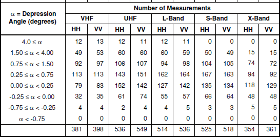
. As an example of the derivation of each value of ![]() provided as modeling information in what follows, Table 5.2 illustrates the like-classified groups of measured clutter histograms for one terrain type—namely, low-relief forest with depression angle from 0.25° to 0.75°. The data in Table 5.2 are separated by frequency band (VHF, UHF, L-, S-, X-bands), range resolution (F = fat = 150 m; T = thin = 36 m for VHF and UHF bands, = 15 m for L-, S-, X-bands), and polarization (V = vertical, H = horizontal).
provided as modeling information in what follows, Table 5.2 illustrates the like-classified groups of measured clutter histograms for one terrain type—namely, low-relief forest with depression angle from 0.25° to 0.75°. The data in Table 5.2 are separated by frequency band (VHF, UHF, L-, S-, X-bands), range resolution (F = fat = 150 m; T = thin = 36 m for VHF and UHF bands, = 15 m for L-, S-, X-bands), and polarization (V = vertical, H = horizontal).
TABLE 5.2
Information* on Patch Values of Mean Clutter Strength ![]() Underlying
Underlying ![]() for Forest/Low-Relief Terrain at 0.25° to 0.75° Depression Angle, by Frequency Band, Range Resolution, and Polarization
for Forest/Low-Relief Terrain at 0.25° to 0.75° Depression Angle, by Frequency Band, Range Resolution, and Polarization

*This table shows the number of patch measurements of ![]() available as a set for each combination of parameters, and various statistical attributes (including the median) of each set.
available as a set for each combination of parameters, and various statistical attributes (including the median) of each set.
Res = range resolution; F = 150m; T = 36m for VHF and UHF, = 15m for L-, S-, X-bands; F+T = both F and T range res. data combined.
Pol = polarization; V+H = both V and H polarization data combined.
Npts = number of clutter patch histograms.
Each line in the table corresponds to one group of like classified histograms. In each line, the following information is provided: the number of histograms in the group (Npts) which is also the number of available like-classified values of clutter patch mean strength in dB; the median of these dB values (which is what is selected for ![]() ); the mean of these dB values; the standard deviation of these dB values (i.e., the 1-σ variability of
); the mean of these dB values; the standard deviation of these dB values (i.e., the 1-σ variability of ![]() ); the maximum of these dB values (the strongest like-classified patch measured); and the minimum of these dB values (the weakest like-classified patch measured). Looking ahead to Table 5.27 in Section 5.4.3.1, the values shown in the 0.25° to 0.75° lines in the upper and lower subtables of Table 5.27 come from Table 5.2. For example, lines 5 and 6 in Table 5.2 provide Npts = 113, 113 (4th column) and
); the maximum of these dB values (the strongest like-classified patch measured); and the minimum of these dB values (the weakest like-classified patch measured). Looking ahead to Table 5.27 in Section 5.4.3.1, the values shown in the 0.25° to 0.75° lines in the upper and lower subtables of Table 5.27 come from Table 5.2. For example, lines 5 and 6 in Table 5.2 provide Npts = 113, 113 (4th column) and ![]() (5th column) for vertical and horizontal polarization, respectively, at VHF. Corresponding information to that shown in Table 5.2 lies behind all terrain type/depression angle categories for which
(5th column) for vertical and horizontal polarization, respectively, at VHF. Corresponding information to that shown in Table 5.2 lies behind all terrain type/depression angle categories for which ![]() values are provided in following Sections 5.3 and 5.4.
values are provided in following Sections 5.3 and 5.4.
TABLE 5.27
Mean Clutter Strength ![]() and Number of Measurements for Low-Relief Forest, by Frequency Band, Polarization, and Depression Anglea
and Number of Measurements for Low-Relief Forest, by Frequency Band, Polarization, and Depression Anglea

aTable 5.24 defines the population of terrain patches upon which these data are based.
5.2.3.2 DERIVATION OF aw RESULTS
The spread in a clutter spatial amplitude distribution as given, for example, by the ratio of standard deviation-to-mean or by the mean-to-median ratio, is fundamentally dependent on radar spatial resolution. Radar spatial resolution A (see Section 2.3.1.1) is given by
where
Δθ = one-way 3-dB azimuth beamwidth.
Like-classified groups of measured clutter histograms were formed in which the classifiers were: terrain type, relief, depression angle, range interval, range resolution, and azimuth beamwidth. Three range intervals were utilized, as: interval 1, 1 to 11.3 km; interval 2, 11.3 to 35.7 km; interval 3, range > 35.7 km. The measured clutter histograms are approximately equally distributed within these three intervals. Two range resolutions are available, wide pulse (i.e., 150 m) or narrow pulse (i.e., 36 m at VHF and UHF, 15 m at L-, S-, and X-bands). Five azimuth beamwidths are available, one per frequency band, as: 13° at VHF, 5° at UHF, 3° at L-band, 1° at S- and X-bands. Although S- and X-bands both have ≈1° azimuth beamwidth, they are kept separate in spread analysis classification grouping to keep the frequency bands separate in the scatter plots (but not in the regression).
For each like-classified group of measured clutter histograms, three parameters were collected from each of the measured clutter histograms within the group. These three parameters are: (1) the ratio of standard deviation-to-mean, (2) the mean-to-median ratio, and (3) the value of spatial resolution A applicable for the measurement. The median values of each of these three parameters were selected as representative values to characterize the spread in that particular like-classified group of measurements. Spread characterization utilizing these three parameters proceeded as follows. For each terrain type/relief/depression angle category, two scatter plots were formed. The first scatter plot shows the ratio of standard deviation-to-mean vs log10 A. The second scatter plot shows the mean-to-median ratio vs log10 A.
Each plotted point in the first of these scatter plots shows the median value of ratio of standard deviation-to-mean vs the median value of log10 A for a particular like-classified group of measured clutter histograms. A number of these scatter plots of standard deviation-to-mean vs log10 A are shown in Sections 5.3 and 5.4, one scatter plot for a selected depression angle regime in each terrain type/relief category. Similar to the first scatter plot, each plotted point in the second scatter plot shows the median value of mean-to-median ratio vs the median value of log10 A for a particular like-classified group of measured clutter histograms. The maximum number of points in a scatter plot is 30 (five azimuth beamwidths, two pulse lengths, three range intervals), but little narrow pulse data is generally available in the third range interval.
Regression analysis was performed in each scatter plot. These regression analyses generally show significantly decreasing spread with decreasing resolution (i.e., increasing A) for each terrain type/relief/depression angle category. The regression line for each scatter plot is provided as modeling information for spread in clutter amplitude distributions in Chapter 5. The regression line is generally characterized by its values at A = 103 m2 and A = 106 m2, with a few noted exceptions.
Modeling information characterizing spread in clutter spatial amplitude distributions based on regression analysis in the scatter plots is provided two ways: (1) based on measured ratios of standard deviation-to-mean and (2) based on measured mean-to-median ratios. For both ways, the regression line values at A = 103 m2 and A = 106 m2 are converted to the corresponding two values of Weibull shape parameter aw at A = 103 m2 and A = 106 m2 by Equations (5.3) and (5.4). These pairs of values of aw are tabulated by terrain type/relief/depression angle category in Sections 5.3 and 5.4. In addition to the paired values of aw, the underlying paired values of ratios of standard deviation-to-mean and mean-to-median ratio are also tabulated. The number of clutter patches and number of measured clutter histograms that each scatter plot (i.e., regression analysis) is based on is also tabulated.
This tabulated modeling information for Weibull shape parameter aw is used as follows. First, the spatial resolution A of the radar under study is calculated at the terrain point under consideration. Then linear interpolation on log10 A between the values of aw at A = 103 m2 and A = 106 m2 for the appropriate terrain type/relief/depression angle category is performed to obtain the value of aw at the radar spatial resolution A in question. Preference is given to the tabulated values of aw based on measured ratios of standard deviation-to-mean. The additional provision of tabulated values of aw based on measured mean-to-median ratios provides a first indication of the degree of validity of modeling the underlying measured data with Weibull statistics, based on how closely aw computed from measured ratios of standard deviation-to-mean approximates aw computed from measured mean-to-median ratios. The like-classified sets of measured clutter histograms, upon which the aw modeling information of Chapter 5 is based, number 1,510. Note that these are different sets than those upon which the ![]() modeling information is based.
modeling information is based.
Information Underlying aw. As described above, the aw values provided as modeling information in what follows come from regression in scatter plots. Two scatter plots were formed: one of sd/mean (dB) vs log10 A; the other of mean/median (dB) vs log10 A. Each scatter plot comes from like-classified groups of measured clutter histograms. As an example of the information underlying the two scatter plots for low-relief forest with depression angle from 0.25° to 0.75°, Table 5.3 is shown here in three parallel parts. Parts (a), (b), and (c) show results for sd/mean (dB), mean/median (dB), and patch mid-range (km), respectively.
TABLE 5.3a
Information* on Patch Values of SD/Mean of σ°F4 Underlying aw for Forest/Low-Relief Terrain at 0.25° to 0.75° Depression Angle, by Frequency Band, Range Resolution, and Range Interval

*This table shows the number of patch measurements of SD/Mean of σ°F4 available as a set for each combination
of parameters, and various statistical attributes (including the median) of each set.
Res = range resolution (m); F = 150m; T = 36m for VHF and UHF, = 15m for L-, S-, X-Bands.
Rng = range interval: 1 (1 to 11.3 km); 2 (11.3 to 35.7 km); 3 (> 35.7 km).
X = log10 (A), A = r Δr Δθ, Δ r = rang. res. (m), Δθ = az. bw. (rad), r = median range (m).
Npts = number of clutter patch histograms.
TABLE 5.3b
Information* on Patch Values of Mean/Median of σ°F4 Underlying aw for Forest/Low-Relief Terrain at 0.25° to 0.75° Depression Angle, by Frequency Band, Range Resolution, and Range Interval

*This table shows the number of patch measurements of Mean/Median of σ°F4 available as a set for each combination of parameters, and various statistical attributes (including the median) of each set.
Res = range resolution (m); F = 150m; T = 36m for VHF and UHF, = 15m for L-, S-, X-Bands.
Rng = range interval: 1 (1 to 11.3 km); 2 (11.3 to 35.7 km); 3 (> 35.7 km).
X = log10 (A), A = r Δr Δθ, Δr = rang. res. (m), Δθ = az. bw. (rad), r = median range (m).
Npts = number of clutter patch histograms.
TABLE 5.3c
Information* on Patch Values of “Mid-Range to Clutter Patch” Underlying the Median Range r and Resolution A Associated with aw for Forest/Low-Relief Terrain at 0.25° to 0.75° Depression Angle, by Frequency Band, Range Resolution, and Range Interval

*This table shows the number of patch measurements of mid-range available as a set for each combination of parameters, and various statistical attributes (including the median) of each set.
Res = range resolution (m); F = 150m; T = 36m for VHF and UHF, = 15m for L-, S-, X-Bands.
Rng = range interval: 1 (1 to 11.3 km); 2 (11.3 to 35.7 km); 3 (> 35.7 km).
X = log10 (A), A = r Δr Δθ, Δr = rang. res. (m), Δθ = az. bw. (rad), r = median range (m).
Npts = number of clutter patch histograms.
Consider first Table 5.3(a) for sd/mean (dB). The data in Table 5.3(a) are separated by frequency band (VHF, UHF, L, S, X), range resolution (Fat or Thin), and range interval (1, 2, or 3, as described previously). Each line in the table corresponds to one group of like-classified histograms and one point in the corresponding scatter plot—note that the groups are different from those of Table 5.2. In each line of Table 5.3(a), the following information is provided: the median value of mid-range cell size A for the group (shown under X as X = log10 A and A = r Δr Δθ in m2); the number of histograms in the group (Npts), which is also the number of available like-classified values of ratio of sd/mean (dB), one from each clutter patch histogram; the median of these dB values of sd/mean (which forms the ordinate of the point in the scatter plot corresponding to this line); the mean of the dB values of sd/mean; the standard deviation of the dB values of sd/mean (i.e., the vertical 1-σ variability of this point in the scatter plot); the maximum of these dB values of sd/mean (i.e., the maximum patch value of sd/mean in this group); and the minimum of these dB values of mean/median. Thus, each line in Table 5.3(a) corresponds to the ordinate of a given point in a given scatter plot. For example, the scatter plot for low-relief forest, 0.0° to 0.25° depression angle is shown as Figure 5.27 in Section 5.4.3.2 (note: the plot corresponding to the 0.25° to 0.75° depression angle regime of Table 5.3 is not shown).

FIGURE 5.27 Ratio of standard deviation-to-mean (SD/Mean) vs radar spatial resolution A for low-relief forest with depression angle between 0.0 and 0.25 degrees.
Table 5.3(b) is similar to Table 5.3(a) except Table 5.3(b) provides underlying information for the ordinate of the plotted points in the scatter plots of mean/median (dB) vs log10 A. Examples of the mean/median scatter plots are not shown in this book; they appear similar to the sd/mean scatter plots, except that they employ a different y-scale.
Table 5.3(c) is similar to Table 5.3(a) except Table 5.3(c) provides underlying information for the abscissas of the plotted points in both kinds of scatter plots. The abscissa is 10log A where A is cell area in m2. As discussed above, A = r·Δr·Δθ where Δr (range resolution) and Δθ (azimuth beamwidth) are fixed within any like-classified group (i.e., any line in the table), but r is the range in km to the center (i.e., mid-range) of each clutter patch in the group. Thus each line in Table 5.3(c) applies to the like-classified set of patch mid-range values, and the median value of mid-range is selected as r in the computation of A and hence the value of X = log10 A shown in each line of Table 5.3(c).
Thus a given point in the scatter plot of sd/mean (dB) vs log10 A for forest/low-relief/depression angle from 0.25° to 0.75° is obtained by selecting the appropriate value of “Median” in Table 5.3(a) as the ordinate, and the corresponding value of X that comes from the corresponding value of “Median” in Table 5.3(c). Scatter plots of sd/mean vs log10 A and mean/median vs log10A were generated for all terrain type/depression angle categories. Each pair of scatter plots came from corresponding information similar to the three parts of Table 5.3. Shape parameter aw data obtained from regression in these scatter plots is provided in Sections 5.3 and 5.4.
5.2.3.3 STATISTICAL CONFIDENCE
In Chapter 5, some clutter modeling results are obtained from many similar measurements leading to high statistical confidence, whereas other results are obtained from fewer measurements leading to less confidence. The rationale followed in Chapter 5 is to present all of the results obtained regardless of the degree of trust, confidence coefficient, or generality associated with each. This is in contrast to the interim clutter model of Chapter 4, Section 4.2, where some smoothing of thinner data was employed. In Chapter 5, information specifying the number of like-classified measurements involved for each ![]() or aw number is included as a means of allowing assessment of statistical validity or generality of the result. Statistical sampling populations and associated confidence levels are usually large in the depression angle regimes near grazing incidence. The sampling populations decrease as depression angle moves to outlying positive or negative depression angle regimes. In the color plots of mean clutter strength
or aw number is included as a means of allowing assessment of statistical validity or generality of the result. Statistical sampling populations and associated confidence levels are usually large in the depression angle regimes near grazing incidence. The sampling populations decrease as depression angle moves to outlying positive or negative depression angle regimes. In the color plots of mean clutter strength ![]() vs frequency, open symbols are occasionally used to indicate
vs frequency, open symbols are occasionally used to indicate ![]() numbers judged likely to be relatively measurement specific and non-representative of the general mean clutter strength applicable to that situation, on the basis of relatively few measurements and clutter strength values far removed from the general trends otherwise observed.
numbers judged likely to be relatively measurement specific and non-representative of the general mean clutter strength applicable to that situation, on the basis of relatively few measurements and clutter strength values far removed from the general trends otherwise observed.
5.2.3.4 USE OF MODELING INFORMATION
The Weibull coefficient modeling information may be employed to generate a σ°F4 clutter strength number (i.e., realization) for a given spatial cell. First, it is determined if the cell is geometrically visible from the antenna position or if the cell is masked or shadowed by intervening terrain of higher elevation. If masked, as a first approximation, zero clutter power is assigned to the cell (the information of this book is not directly applicable to shadowed cells; but see Appendix 4.D). If visible, the depression angle from the antenna position to the cell is computed, the terrain type and relief for the cell is determined, and the radar spatial resolution A at the cell is calculated. This determination of terrain type/relief/depression angle/spatial resolution for the cell leads to the pair of Weibull coefficients, ![]() , aw, which specify the clutter amplitude distribution for that combination of terrain type, relief, depression angle, and resolution. A single random variate from this clutter amplitude distribution is assigned as clutter strength to the cell under examination. The modeler then proceeds to the next cell and repeats the process. In this manner, all visible cells at the site are assigned Weibull random variates as clutter strength, each appropriate to the radar parameters, geometry, and terrain type for the cell under consideration. The cell-to-cell spatial correlation that occurs in this process is that provided by the underlying land cover and DTED information; otherwise, the random variates of clutter strength occur independently from cell to cell, as indeed for the most part do the measured data (see Chapter 4, Section 4.6.3). Further explanation of this terrain-specific modeling rationale is provided in Chapter 4. Techniques for validating and improving this approach to clutter modeling are briefly described in Section 5.5.
, aw, which specify the clutter amplitude distribution for that combination of terrain type, relief, depression angle, and resolution. A single random variate from this clutter amplitude distribution is assigned as clutter strength to the cell under examination. The modeler then proceeds to the next cell and repeats the process. In this manner, all visible cells at the site are assigned Weibull random variates as clutter strength, each appropriate to the radar parameters, geometry, and terrain type for the cell under consideration. The cell-to-cell spatial correlation that occurs in this process is that provided by the underlying land cover and DTED information; otherwise, the random variates of clutter strength occur independently from cell to cell, as indeed for the most part do the measured data (see Chapter 4, Section 4.6.3). Further explanation of this terrain-specific modeling rationale is provided in Chapter 4. Techniques for validating and improving this approach to clutter modeling are briefly described in Section 5.5.
For those interested in general clutter levels (e.g., means, medians) exclusive of cell-to-cell variability, use of the modeling information provided in Chapter 5 is more direct. Mean clutter strength is σwodirectly tabulated. Median clutter strength σ°50 and other percentile levels and moments are dependent on radar spatial resolution A. Median clutter strength σ°50 is simply calculated from ![]() and the mean-to-median ratio; the mean-to-median ratio may be obtained for the radar resolution A under consideration by linear interpolation on log10 A between tabulated values at A = 103 m2 and A = 106 m2. The standard deviation may be obtained in a manner directly parallel to that by which the median is obtained. Other percentile levels may be simply calculated from the Weibull cumulative distribution function [Eq. (5.2)].
and the mean-to-median ratio; the mean-to-median ratio may be obtained for the radar resolution A under consideration by linear interpolation on log10 A between tabulated values at A = 103 m2 and A = 106 m2. The standard deviation may be obtained in a manner directly parallel to that by which the median is obtained. Other percentile levels may be simply calculated from the Weibull cumulative distribution function [Eq. (5.2)].
5.2.3.5 PRESENTATION OF MATERIAL
Sections 5.3 and 5.4 provide extensive modeling information for low-angle land clutter spatial amplitude statistics within a standard presentation format. The format utilized follows that of the interim clutter model presented in Chapter 4, Section 4.2, and illustrated in Figure 4.3. The format of presentation of mean clutter strength ![]() is reviewed here as an aid to the presentation of the extensive modeling information that directly follows.
is reviewed here as an aid to the presentation of the extensive modeling information that directly follows.
The clutter modeling information that follows is based on depression angle. Figure 5.6 shows depression angle to be the angle below the horizontal from the radar to the backscattering terrain point. A precise mathematical definition of depression angle is given by Equation (5.1); see also Appendix 2.C of Chapter 2. As shown in Figure 5.6, terrain can occasionally rise to elevations higher than the radar which leads to negative depression angle. Approximately 30% of the clutter modeling information to follow applies to clutter measurements obtained at negative depression angle.
The clutter modeling information that follows is presented within bins (i.e., narrow angular regimes) of depression angle. The depression angle bins utilized are shown in Table 5.4. As is apparent in Table 5.4, different binning is utilized in low-relief terrain (terrain slopes < sin 2°) than in high-relief terrain (terrain slopes > 2°). In low-relief terrain, five positive and three negative depression angle bins are used; in high-relief terrain, five positive and two negative bins are used. The bins are very narrow, particularly at low depression angle, and more so for low-relief than high-relief terrain. Each bin typically contains hundreds of clutter measurements. What is plotted is the median value of clutter patch mean strength ![]() within each bin.
within each bin.
It will be seen in the clutter modeling information to follow that, as a result of medianizing over many measurements, the small differences in depression angle shown in Table 5.4 can account for systematic differences in mean clutter strength that in total can cover wide ranges. The bins are shown color-coded in Table 5.4; the same color coding is used in plotting mean clutter strength σwo in color figures to follow, with different shaped symbols used to plot ![]() at VV-polarization (circles) and HH-polarization (squares). The color codes are as follows: for increasing positive depression angle, cyan, dark blue, purple, magenta, red for bins 1 to 5, respectively; for increasing negative depression angle, dark green, intermediate green, light green for bins −1, −2, and −3 in low-relief terrain, and dark green, intermediate green for bins −1, −2 in high-relief terrain, respectively. The category of long-range mountains requires a specialized negative depression angle category. Complete data are not always available for all terrain types at outlying depression angles.
at VV-polarization (circles) and HH-polarization (squares). The color codes are as follows: for increasing positive depression angle, cyan, dark blue, purple, magenta, red for bins 1 to 5, respectively; for increasing negative depression angle, dark green, intermediate green, light green for bins −1, −2, and −3 in low-relief terrain, and dark green, intermediate green for bins −1, −2 in high-relief terrain, respectively. The category of long-range mountains requires a specialized negative depression angle category. Complete data are not always available for all terrain types at outlying depression angles.
In the clutter modeling information that follows, for each terrain type mean clutter strength ![]() is plotted vs radar frequency against a log-frequency x-axis in order to show results for all five frequency bands together. The plotting methodology is shown representationally in the diagram of Figure 5.7. Within each frequency band,
is plotted vs radar frequency against a log-frequency x-axis in order to show results for all five frequency bands together. The plotting methodology is shown representationally in the diagram of Figure 5.7. Within each frequency band, ![]() results separated by depression angle bin are plotted by slightly displacing the plot symbols horizontally from bin to bin to avoid symbol overlap. This plot methodology, covering eight depression angle bins, is shown for X-band in an exaggerated way in the diagram of Figure 5.7. The sequential horizontal displacements shown in Figure 5.7 do not imply an in-band frequency shift; the cluster of sixteen plotted values of
results separated by depression angle bin are plotted by slightly displacing the plot symbols horizontally from bin to bin to avoid symbol overlap. This plot methodology, covering eight depression angle bins, is shown for X-band in an exaggerated way in the diagram of Figure 5.7. The sequential horizontal displacements shown in Figure 5.7 do not imply an in-band frequency shift; the cluster of sixteen plotted values of ![]() shown in Figure 5.7 all apply for a single X-band frequency. Similar bin-to-bin horizontal offsetting of plot symbols is also employed in the lower four bands.
shown in Figure 5.7 all apply for a single X-band frequency. Similar bin-to-bin horizontal offsetting of plot symbols is also employed in the lower four bands.

FIGURE 5.7 Five-frequency plot methodology showing depression angle color coding. Circles represent VV-polarization; squares represent HH-polarization. Each plot symbol is a median value of mean clutter strength over many clutter patch measurements.
Mean clutter strength ![]() generally increases both with increasing positive depression angle and with increasing negative depression angle. As a result, the in-band clusters of plotted data in multiple depression angle bins often take on the v-shape shown representatively by the X-band cluster in Figure 5.7. Thus, as a point of departure in interpreting the results, it is suggested that the reader first look for v-shapes indicating whether or not consistent depression angle effects on clutter strength occur for the particular frequency band and terrain type of interest.
generally increases both with increasing positive depression angle and with increasing negative depression angle. As a result, the in-band clusters of plotted data in multiple depression angle bins often take on the v-shape shown representatively by the X-band cluster in Figure 5.7. Thus, as a point of departure in interpreting the results, it is suggested that the reader first look for v-shapes indicating whether or not consistent depression angle effects on clutter strength occur for the particular frequency band and terrain type of interest.
5.3 LAND CLUTTER COEFFICIENTS FOR GENERAL TERRAIN
A radar designer or analyst may often require that the characteristics of land clutter be specified independently of specific terrain type. There are two reasons for this requirement. First, most radars must maintain performance when sited in various terrains and situations. Second, even at individual sites much clutter producing terrain is often composite and mixed over scales of several kilometers. In Section 5.3, modeling information characterizing low-angle land clutter spatial amplitude distributions is provided based on a large set of 30,246 measured clutter histograms from 1,628 clutter patches classified as general mixed rural. These measurements comprise 51% of the multifrequency Phase One clutter measurement data. This set of measurements includes the measurements from all mixed terrain types except those primarily classified as urban. Mixed terrain is generally neither completely open nor completely tree-covered. Because of the large amount of composite terrain clutter measurement data upon which they are based, the results of Section 5.3 are very general. General effects of depression angle, terrain relief, radar frequency, polarization, and resolution are quantified independent of specific terrain type.
5.3.1 GENERAL MIXED RURAL TERRAIN
5.3.1.1 High-Relief General Mixed Rural Terrain
Table 5.5 shows the number of patches and measured clutter histograms by depression angle regime and terrain relief for general mixed rural terrain. Table 5.6 presents Weibull mean clutter strength ![]() for general mixed rural terrain of high relief, by depression angle, frequency band, and polarization. The number of measured clutter histograms upon which each value of
for general mixed rural terrain of high relief, by depression angle, frequency band, and polarization. The number of measured clutter histograms upon which each value of ![]() in Table 5.6 is based is also presented in the lower of the two subtables comprising Table 5.6. High-relief terrain has terrain slopes > 2°. The
in Table 5.6 is based is also presented in the lower of the two subtables comprising Table 5.6. High-relief terrain has terrain slopes > 2°. The ![]() data of Table 5.6 are plotted in Figure 5.8. To avoid obscuring results with overlapping plot symbols, within each frequency band in Figure 5.8 the colored plot symbols are plotted with small increasing horizontal displacements to the right as depression angle decreases from its highest positive regime through zero to its highest negative regime (i.e., top to bottom in Table 5.6). These small artificial displacements do not indicate an in-band frequency shift.
data of Table 5.6 are plotted in Figure 5.8. To avoid obscuring results with overlapping plot symbols, within each frequency band in Figure 5.8 the colored plot symbols are plotted with small increasing horizontal displacements to the right as depression angle decreases from its highest positive regime through zero to its highest negative regime (i.e., top to bottom in Table 5.6). These small artificial displacements do not indicate an in-band frequency shift.
TABLE 5.5
Numbers of Terrain Patches and Measured Clutter Histograms for General Mixed Rural Terrain, by Relief and Depression Anglea,b,c

aMixed terrain implies primary and secondary terrain classification. Rural terrain includes all classes except urban.
bA terrain patch is a land surface macroregion usually several kms on a side (median patch area = 12.62 km2).
cA measured clutter histogram contains all of the temporal (pulse by pulse) and spatial (resolution cell by resolution cell) clutter samples obtained in a given measurement of a terrain patch. A terrain patch was usually measured many times (nominally 20) as RF frequency (5), polarization (2), and range resolution (2) were varied over the Phase One radar parameter matrix.
TABLE 5.6
Mean Clutter Strength ![]() and Number of Measurements for General Mixed Rural Terrain of High Relief, by Frequency Band, Polarization, and Depression Anglea
and Number of Measurements for General Mixed Rural Terrain of High Relief, by Frequency Band, Polarization, and Depression Anglea


aTable 5.5 defines the population of terrain patches upon which these data are based.

In each frequency band of Figure 5.8, the resultant set of colored plot symbols has a v-shape. The consistent v-shape indicates consistent depression angle effects in each band, where ![]() increases with both increasing positive (left side of v-shape, cyan through magenta) and increasing negative (right side of v-shape, dark green through intermediate green) depression angle. In what follows in Chapter 5, the
increases with both increasing positive (left side of v-shape, cyan through magenta) and increasing negative (right side of v-shape, dark green through intermediate green) depression angle. In what follows in Chapter 5, the ![]() data for each terrain type are plotted in a figure in which the manner of data presentation is similar to that employed in Figure 5.8.
data for each terrain type are plotted in a figure in which the manner of data presentation is similar to that employed in Figure 5.8.
The cyan (i.e., light blue) colored symbols in Figure 5.8 represent the lowest positive depression angle regime (0° to 1°) in high-relief terrain. These results are based on a significantly larger number of measurements than the other depression angle regimes in
Table 5.6 and hence may be regarded as the most reliable data shown in Figure 5.8. In moving from cyan through the higher positive depression angles in Figure 5.8, there is a monotonic rise up the left side of the v-shaped cluster from cyan to dark blue (1° to 2°) to purple (2° to 4°) to magenta (4° to 6°). Thus in each frequency band Figure 5.8 shows a strong monotonic increase in ![]() with increasing positive depression angle. The number of measurements falls off with increasing positive or negative depression angle (see Table 5.5). No data are available for depression angle > 6° (red) in any band in Figure 5.8, and no data are available from 4° to 6° (magenta) at S- and X-bands in Figure 5.8 due to the limited Phase One elevation beamwidths in those bands (see Appendix 3.A).
with increasing positive depression angle. The number of measurements falls off with increasing positive or negative depression angle (see Table 5.5). No data are available for depression angle > 6° (red) in any band in Figure 5.8, and no data are available from 4° to 6° (magenta) at S- and X-bands in Figure 5.8 due to the limited Phase One elevation beamwidths in those bands (see Appendix 3.A).
Values of ![]() for negative depression angle are plotted in shades of green. Negative depression angle occurs when steep terrain is observed by the radar at elevations above the antenna. The darkest shade of green shows results in the lowest negative depression angle regime, which is 0° to −1° in high-relief terrain. These dark green (0° to −1°) results in Figure 5.8 are generally close to and usually slightly higher than the cyan (0° to 1°) results, as intuitively would be expected. The shade of green becomes lighter with increasing negative depression angle. In high-relief terrain, only one additional negative depression angle regime is utilized, for depression angle < −1° (intermediate green in Figure 5.8). In every band, the intermediate green values of
for negative depression angle are plotted in shades of green. Negative depression angle occurs when steep terrain is observed by the radar at elevations above the antenna. The darkest shade of green shows results in the lowest negative depression angle regime, which is 0° to −1° in high-relief terrain. These dark green (0° to −1°) results in Figure 5.8 are generally close to and usually slightly higher than the cyan (0° to 1°) results, as intuitively would be expected. The shade of green becomes lighter with increasing negative depression angle. In high-relief terrain, only one additional negative depression angle regime is utilized, for depression angle < −1° (intermediate green in Figure 5.8). In every band, the intermediate green values of ![]() in Figure 5.8 are significantly stronger than the dark green values, thus providing the right sides of the v-shaped clusters.
in Figure 5.8 are significantly stronger than the dark green values, thus providing the right sides of the v-shaped clusters.
There is a general trend of decreasing ![]() with increasing radar carrier frequency in Figure 5.8. At the lowest (positive or negative) depression angles, this trend is slight (e.g., for cyan, 0° to 1°, UHF, L-, and X-band results are all remarkably close in the −29 dB vicinity, with VHF slightly stronger and S-band slighter weaker). At higher (positive or negative) depression angles, the trend is stronger. This trend is largely due to increasing absorption of radio frequency (RF) power from the incident radar wave by tree foliage, VHF to S-band (see Chapter 3). Mixed rural terrain of high relief has a larger component of trees than at low relief. At the highest positive depression angles (magenta and purple) in Figure 5.8, the variation of
with increasing radar carrier frequency in Figure 5.8. At the lowest (positive or negative) depression angles, this trend is slight (e.g., for cyan, 0° to 1°, UHF, L-, and X-band results are all remarkably close in the −29 dB vicinity, with VHF slightly stronger and S-band slighter weaker). At higher (positive or negative) depression angles, the trend is stronger. This trend is largely due to increasing absorption of radio frequency (RF) power from the incident radar wave by tree foliage, VHF to S-band (see Chapter 3). Mixed rural terrain of high relief has a larger component of trees than at low relief. At the highest positive depression angles (magenta and purple) in Figure 5.8, the variation of ![]() with radar frequency f VHF to S-band is approximately
with radar frequency f VHF to S-band is approximately ![]() . In the historical literature, what little information is available on the subject usually suggests a slight trend of increasing clutter strength with increasing radar frequency, for example,
. In the historical literature, what little information is available on the subject usually suggests a slight trend of increasing clutter strength with increasing radar frequency, for example, ![]() or
or ![]() . Thus the trend of decreasing clutter strength with increasing radar frequency seen in many of the Phase One high-angle forest measurements is relatively unexpected. Note that at all positive depression angles in Figure 5.8, the trend of decreasing
. Thus the trend of decreasing clutter strength with increasing radar frequency seen in many of the Phase One high-angle forest measurements is relatively unexpected. Note that at all positive depression angles in Figure 5.8, the trend of decreasing ![]() with increasing radar frequency from VHF to S-band reverses from S-band to X-band. That is, at all positive depression angles there is an S-band dip between L-band and X-band in Figure 5.8, indicating that over the range of frequencies shown, maximum RF absorption occurs at S-band. It is probably not entirely coincidental that S-band is also the frequency band in which the common household microwave oven operates (at 2.45 GHz). In Figure 5.8, the differences with polarization are generally small, on the order of several dB or less, with vertical polarization (VV) almost always stronger than horizontal (HH).
with increasing radar frequency from VHF to S-band reverses from S-band to X-band. That is, at all positive depression angles there is an S-band dip between L-band and X-band in Figure 5.8, indicating that over the range of frequencies shown, maximum RF absorption occurs at S-band. It is probably not entirely coincidental that S-band is also the frequency band in which the common household microwave oven operates (at 2.45 GHz). In Figure 5.8, the differences with polarization are generally small, on the order of several dB or less, with vertical polarization (VV) almost always stronger than horizontal (HH).
Table 5.7 presents the Weibull shape parameter aw and ratios of standard deviation-to-mean and mean-to-median for general mixed rural terrain of high relief, by depression angle and radar spatial resolution. Whereas the information of Table 5.6 specifies the mean or first moment of the clutter spatial amplitude distribution, the information of Table 5.7 specifies the spread or variability in the distribution as determined by the second moment or other derivative quantities. Table 5.5 shows the number of terrain patches and number of measured clutter histograms for general mixed rural terrain of high relief, broken down by depression angle in a parallel manner to that of Table 5.7; that is, the statistical populations underlying the data of Table 5.7 are available in Table 5.5. The numbers of measured clutter histograms in Table 5.5 are further broken down by frequency band and polarization in Table 5.6. Table 5.5 shows no data available for depression angle > 6° for general mixed rural terrain of high relief. Generally, there is little Phase One data available at such a high depression angle, although Section 5.4 shows that there is one high-relief forest clutter patch and six mountain clutter patches at depression angles > 6°.
TABLE 5.7
Shape Parameter aw and Ratios of Standard Deviation-to-Mean (SD/Mean) and Mean-to-Median for General Mixed Rural Terrain of High Relief, by Spatial Resolution A and Depression Anglea


aTable 5.5 defines the population of terrain patches and measurements upon which these data are based.
In Table 5.7, aw is calculated two ways: (1) from the ratio of standard deviation-to-mean and (2) from the mean-to-median ratio. In Table 5.7, and in general throughout Chapter 5, no major systematic difference results between these two methods of calculation of aw, or, including as a third alternative, in the aw that comes from the least-mean-squares best-fitting true Weibull distribution that is matched to the measured distribution over a large central part (i.e., noise level to 0.999 cumulative probability) of the measured distribution. However, aw results by two different methods of calculation are shown in Table 5.7 and in all similar tables throughout Chapter 5 as a first indication of the degree to which Weibull statistics approximate the characteristics of the measured distributions; if the measured distributions were exactly Weibull, the two different methods of calculation of aw would yield identical results.
Each pair of aw numbers in Table 5.7 comes from a scatter plot in which each individual point plotted shows the median value of spread vs the median value of spatial resolution in a group of like-classified measured clutter histograms. For example, for Table 5.7 the standard deviation-to-mean scatter plot for the 2° to 4° depression angle regime is shown in
Figure 5.9. This scatter plot is based on 51 terrain patches and 987 measured clutter histograms, as indicated in Table 5.5. Twelve similar scatter plots underlie the 12 pairs of aw numbers in Table 5.7.
The major parametric variation of aw in Table 5.7 is with radar spatial resolution. In every case, aw is much greater at 103 m2 resolution than at 106 m2 resolution. There is also a weaker trend in Table 5.7 whereby aw decreases as depression angle increases from the 0° to 1° regime (more so with increasing positive depression angle than with increasing negative depression angle). For cell-by-cell Weibull random clutter strength numbers, aw for the radar spatial resolution at the cell under consideration is required. The value of aw applicable at resolution A is obtained by linear interpolation on log10A between the tabulated values of aw at A = 103 m2 and A = 106 m2 shown in Table 5.7. For example, in general mixed rural terrain of high relief in the depression angle regime from 1° to 2°, the applicable value of aw at A = 104 m2 based on: (1) measured ratios of standard deviation-to-mean is aw = 2.53, (2) measured mean-to-median ratios is aw = 2.77, and (3) equal weighting of ratios of standard deviation-to-mean and mean-to-median is aw = 2.65.
The lower subtable of Table 5.7 shows the ratios of standard deviation-to-mean and mean-to-median from which the aw numbers in the upper subtable come. The large spreads in low-angle land clutter spatial amplitude distributions at high spatial resolution are perhaps more dramatically evidenced by these lower numbers (e.g., mean-to-median ratio = 18.9 dB at 103 m2, compared to 6.3 dB at 106 m2, Table 5.7, depression angle regime from 1° to 2°). Figure 5.5 allows quick conversion between the numbers in the upper and lower subtables of Table 5.7, and similar tables throughout Chapter 5. Interpolation in these lower numbers directly yields general second moment or median values at the spatial resolution under consideration. For example, at A = 104 m2, for general mixed rural terrain of high relief in the 1° to 2° depression angle regime, the ratio of standard deviation-to-mean is 5.0 dB and the mean-to-median ratio is 11.7 dB. The applicable mean level ![]() is obtained from Table 5.6. If L-band and vertical polarization happen to be the frequency and polarization of the radar in question, then, continuing the example, in general mixed rural terrain of high relief in the 1° to 2° depression angle regime at spatial resolution of 104 m2, the applicable low-angle land clutter spatial amplitude distribution has
is obtained from Table 5.6. If L-band and vertical polarization happen to be the frequency and polarization of the radar in question, then, continuing the example, in general mixed rural terrain of high relief in the 1° to 2° depression angle regime at spatial resolution of 104 m2, the applicable low-angle land clutter spatial amplitude distribution has ![]() ,
, ![]() , and standard deviation equal to −21.0 dB.
, and standard deviation equal to −21.0 dB.
5.3.1.2 LOW-RELIEF GENERAL MIXED RURAL TERRAIN
Table 5.8 presents Weibull mean clutter strength ![]() for general mixed rural terrain of low relief by depression angle, frequency band, and polarization. The lower of the two subtables comprising Table 5.8 shows the number of measurements upon which each
for general mixed rural terrain of low relief by depression angle, frequency band, and polarization. The lower of the two subtables comprising Table 5.8 shows the number of measurements upon which each ![]() value in the upper subtable is based. Low-relief terrain has terrain slopes < 2°. Table 5.5 indicates that, within the Phase One general mixed rural clutter data, low relief occurs somewhat more frequently (viz., 56%) than high relief (viz., 44%).
value in the upper subtable is based. Low-relief terrain has terrain slopes < 2°. Table 5.5 indicates that, within the Phase One general mixed rural clutter data, low relief occurs somewhat more frequently (viz., 56%) than high relief (viz., 44%).
TABLE 5.8
Mean Clutter Strength ![]() and Number of Measurements for General Mixed Rural Terrain of Low Relief, by Frequency Band, Polarization, and Depression Anglea
and Number of Measurements for General Mixed Rural Terrain of Low Relief, by Frequency Band, Polarization, and Depression Anglea


aTable 5.5 defines the population of terrain patches upon which these data are based.
The low-relief ![]() data of Table 5.8 are plotted in Figure 5.10 in a manner similar to that employed with the high-relief
data of Table 5.8 are plotted in Figure 5.10 in a manner similar to that employed with the high-relief ![]() data in Figure 5.8. As in Figure 5.8, in each frequency band of Figure 5.10 the set of colored plot symbols continues to have a consistent v-shape indicating consistent depression angle effects in each band. The v-shapes of the low-relief data in Figure 5.10 are, however, considerably more pronounced than those of the high-relief data in Figure 5.8. That is, depression angle effects are stronger at low relief than at high relief.
data in Figure 5.8. As in Figure 5.8, in each frequency band of Figure 5.10 the set of colored plot symbols continues to have a consistent v-shape indicating consistent depression angle effects in each band. The v-shapes of the low-relief data in Figure 5.10 are, however, considerably more pronounced than those of the high-relief data in Figure 5.8. That is, depression angle effects are stronger at low relief than at high relief.

The cyan colored symbols in Figure 5.10 represent the lowest positive depression angle regime (0° to 0.25°) in low-relief terrain and are based on a large number of measurements (see Table 5.8). In moving from cyan through the higher positive depression angles in Figure 5.10, in general there is a monotonic rise (with a few minor exceptions) up the left side of the v-shaped cluster from cyan to dark blue (0.25° to 0.75°) to purple (0.75° to 1.5°) to magenta (1.5° to 4°) to red (depression angle > 4°). Thus in each frequency band Figure 5.10 shows a strong increase in ![]() with increasing positive depression angle. The number of measurements falls off at outlying positive and negative depression angles (see Tables 5.5 and 5.8). No data are available for depression angle > 4° (red) at S- and X-bands in Figure 5.10 due to the limited Phase One elevation beamwidths in those bands.
with increasing positive depression angle. The number of measurements falls off at outlying positive and negative depression angles (see Tables 5.5 and 5.8). No data are available for depression angle > 4° (red) at S- and X-bands in Figure 5.10 due to the limited Phase One elevation beamwidths in those bands.
Values of ![]() for negative depression angle are plotted in shades of green. The darkest shade of green shows results in the lowest negative depression angle regime, which is 0° to −0.25° in low-relief terrain. These dark green (0° to −0.25°) results in Figure 5.10 are generally close to and usually slightly higher than the cyan (0° to 0.25°) results. The shade of green becomes lighter with increasing negative depression angle. In low-relief terrain, two additional negative depression angle regimes are utilized for depression angles from −0.25° to −0.75° (intermediate green) and for depression angles < −0.75° (light green). In moving from cyan through the three green negative depression angle regimes in Figure 5.10, in general there is a strong monotonic rise (with two minor exceptions) up the right side of each v-shaped cluster.
for negative depression angle are plotted in shades of green. The darkest shade of green shows results in the lowest negative depression angle regime, which is 0° to −0.25° in low-relief terrain. These dark green (0° to −0.25°) results in Figure 5.10 are generally close to and usually slightly higher than the cyan (0° to 0.25°) results. The shade of green becomes lighter with increasing negative depression angle. In low-relief terrain, two additional negative depression angle regimes are utilized for depression angles from −0.25° to −0.75° (intermediate green) and for depression angles < −0.75° (light green). In moving from cyan through the three green negative depression angle regimes in Figure 5.10, in general there is a strong monotonic rise (with two minor exceptions) up the right side of each v-shaped cluster.
At VHF in Figure 5.10, at low depression angles (e.g., cyan, 0° to 0.25°) clutter strengths are low due to multipath loss over the open components of the low-relief mixed rural terrain—this effect is not at work in the high-relief data of Figure 5.8. Remaining with VHF in Figure 5.10, at high depression angles (e.g., red, > 4°) clutter strengths are high because of the low RF absorption at VHF by the forested components of the low-relief mixed rural terrain—this effect is at work in the high-relief data of Figure 5.8. As a result of these two effects, the amplitude of the v-shaped cluster of plot symbols at VHF in Figure 5.10 is wide, viz., 24 dB, compared to 13 dB in Figure 5.8. These are the ranges over which small changes in depression angle affect the mean strength ![]() of land clutter at VHF in general mixed rural terrain of low and high relief, respectively. In Figure 5.10, as radar carrier frequency f rises from VHF into the microwave regime, at low depression angle (cyan)
of land clutter at VHF in general mixed rural terrain of low and high relief, respectively. In Figure 5.10, as radar carrier frequency f rises from VHF into the microwave regime, at low depression angle (cyan) ![]() rises from VHF to L-band due to decreasing multipath loss with approximate dependence
rises from VHF to L-band due to decreasing multipath loss with approximate dependence ![]() , whereas at high depression angle (red and magenta) wo (f) falls from VHF to S-band due to increasing RF absorption by tree foliage with approximate dependence
, whereas at high depression angle (red and magenta) wo (f) falls from VHF to S-band due to increasing RF absorption by tree foliage with approximate dependence ![]() . At intermediate depression angles, the variation with radar frequency is intermediate between these extremes. As a result of these two opposite trends with radar frequency, the data points plotted in Figure 5.10 take on a funnel shape. As in the high-relief data of Figure 5.8, there is an S-band dip between L-band and X-band in the low-relief data of Figure 5.10, with the dip more pronounced at high depression angle (magenta) than at low depression angle (cyan). This dip occurs at all positive depression angles in Figure 5.10. As in Figure 5.8 at high relief, in Figure 5.10 at low relief the differences with polarization are generally small, on the order of several dB or less, with vertical polarization (VV) almost always stronger than horizontal (HH).
. At intermediate depression angles, the variation with radar frequency is intermediate between these extremes. As a result of these two opposite trends with radar frequency, the data points plotted in Figure 5.10 take on a funnel shape. As in the high-relief data of Figure 5.8, there is an S-band dip between L-band and X-band in the low-relief data of Figure 5.10, with the dip more pronounced at high depression angle (magenta) than at low depression angle (cyan). This dip occurs at all positive depression angles in Figure 5.10. As in Figure 5.8 at high relief, in Figure 5.10 at low relief the differences with polarization are generally small, on the order of several dB or less, with vertical polarization (VV) almost always stronger than horizontal (HH).
Comparison of Figures 5.8 and 5.10 indicates that there exist considerable differences in mean clutter strength ![]() between general mixed rural terrain of high relief (terrain slopes > 2°) and low relief (terrain slopes < 2°), respectively. A major reason for this is that low-relief mixed rural terrain allows multipath propagation to occur, which drives down clutter strengths at low depression angle in the lower bands. Multipath propagation does not occur to any significant degree in high-relief terrain or at high depression angles in low-relief terrain. At high depression angles in the lower bands and at all depression angles in the upper bands, mean clutter strengths in high-relief terrain are somewhat greater than in low-relief terrain, within similar depression angle regimes. Such differences are due directly to the effect of terrain relief on intrinsic σ°; they are less than the low depression angle differences in the lower bands caused by multipath. A contributing factor to all the differences in mean clutter strength with terrain relief indicated in Figures 5.8 and 5.10 is that high-relief mixed rural terrain tends to be somewhat more forested whereas low-relief mixed rural terrain tends to be somewhat more open. Classification by terrain relief in two major regimes as shown in Figures 5.8 and 5.10 is a simple and practicable approach for sorting out the complex phenomenological influences at work in low-angle land clutter.
between general mixed rural terrain of high relief (terrain slopes > 2°) and low relief (terrain slopes < 2°), respectively. A major reason for this is that low-relief mixed rural terrain allows multipath propagation to occur, which drives down clutter strengths at low depression angle in the lower bands. Multipath propagation does not occur to any significant degree in high-relief terrain or at high depression angles in low-relief terrain. At high depression angles in the lower bands and at all depression angles in the upper bands, mean clutter strengths in high-relief terrain are somewhat greater than in low-relief terrain, within similar depression angle regimes. Such differences are due directly to the effect of terrain relief on intrinsic σ°; they are less than the low depression angle differences in the lower bands caused by multipath. A contributing factor to all the differences in mean clutter strength with terrain relief indicated in Figures 5.8 and 5.10 is that high-relief mixed rural terrain tends to be somewhat more forested whereas low-relief mixed rural terrain tends to be somewhat more open. Classification by terrain relief in two major regimes as shown in Figures 5.8 and 5.10 is a simple and practicable approach for sorting out the complex phenomenological influences at work in low-angle land clutter.
Table 5.9 presents the Weibull shape parameter aw and ratios of standard deviation-to-mean and mean-to-median for clutter amplitude distributions in general mixed rural terrain of low relief, by depression angle and radar spatial resolution. The statistical populations underlying the data of Table 5.9 are available in Table 5.5. In Table 5.9, aw is calculated two ways: (1) from the ratio of standard deviation-to-mean and (2) from the mean-to-median ratio. Many of the corresponding aw numbers resulting from these two methods of calculation are remarkably close in Table 5.9. Each pair of aw numbers in Table 5.9 comes from a scatter plot in which each individual point plotted shows the median value of spread vs the median value of spatial resolution in a group of like-classified measured clutter histograms. The standard deviation-to-mean scatter plot for the 0.25° to 0.75° depression angle regime in Table 5.9 is shown in Figure 5.11. The major parametric variation of aw in Table 5.9 is with radar spatial resolution. In every case, aw is much greater at 103 m2 resolution than at 106 m2 resolution. There is a weak trend in Table 5.9 whereby aw decreases as depression angle increases from the 0° to 0.25° regime. There is little indication for aw in terrain of high relief as shown in Table 5.7 to be lower than in terrain of low relief as shown in Table 5.9, as might be expected in these results. The lower subtable of Table 5.9 shows the ratios of standard deviation-to-mean and mean-to-median from which the aw numbers in the upper subtable come. The large spreads in low-angle land clutter spatial amplitude distributions at high spatial resolution continue to be dramatically evidenced by these lower numbers.


5.3.2 FURTHER REDUCTION
The previous results of Section 5.3, although applicable to a single generic terrain type (viz., mixed rural), still require specification of the relief of the terrain (in two categories, viz., high- and low-) and the depression angle at which the terrain is illuminated. A clutter modeler who is unable to specify terrain relief and depression angle may desire that the Phase One clutter measurement data be reduced so as to average together all variations of terrain relief and depression angle. The results of such reduction are presented in what follows. Table 5.10 shows mean clutter strength σwo for general mixed rural terrain by frequency band and polarization, in which all variations with relief and depression angle are subsumed. The ![]() results of Table 5.10 are plotted in Figure 5.12. The lower subtable of Table 5.10 shows that the number of measurements upon which the mean clutter strength results in Table 5.10 are based is large—on the order of 3,000 measurements for each value of
results of Table 5.10 are plotted in Figure 5.12. The lower subtable of Table 5.10 shows that the number of measurements upon which the mean clutter strength results in Table 5.10 are based is large—on the order of 3,000 measurements for each value of ![]() .
.
TABLE 5.10
Mean Clutter Strength ![]() and Number of Measurements for General Mixed Rural Terrain by Frequency Band and Polarization, Inclusive of Variations with Relief and Depression Anglea
and Number of Measurements for General Mixed Rural Terrain by Frequency Band and Polarization, Inclusive of Variations with Relief and Depression Anglea


aTable 5.5 defines the population of terrain patches upon which these data are based.

FIGURE 5.12 Mean clutter strength ![]() vs frequency for general mixed rural terrain, inclusive of variations with relief and depression angle.
vs frequency for general mixed rural terrain, inclusive of variations with relief and depression angle.
The ![]() results of Table 5.10 and Figure 5.12 hover around −30 dB in all five frequency bands and at both polarizations. There is a slight (∼2 dB) S-band dip between L-band and X-band; also, results at vertical polarization are usually slightly stronger (on the order of 1 or 2 dB) than at horizontal polarization (except at L-band where
results of Table 5.10 and Figure 5.12 hover around −30 dB in all five frequency bands and at both polarizations. There is a slight (∼2 dB) S-band dip between L-band and X-band; also, results at vertical polarization are usually slightly stronger (on the order of 1 or 2 dB) than at horizontal polarization (except at L-band where ![]() ). Such differences with frequency and polarization are small. That is, after incorporating all variations with relief and depression angle, mean clutter strength in general mixed rural terrain is remarkably invariant with frequency and polarization. The results of Table 5.10 and Figure 5.12 corroborate corresponding results obtained with repeat sector data in Chapter 3 (cf. Table 3.7 and Figure 3.40).
). Such differences with frequency and polarization are small. That is, after incorporating all variations with relief and depression angle, mean clutter strength in general mixed rural terrain is remarkably invariant with frequency and polarization. The results of Table 5.10 and Figure 5.12 corroborate corresponding results obtained with repeat sector data in Chapter 3 (cf. Table 3.7 and Figure 3.40).
Table 5.11 presents the Weibull shape parameter aw and ratios of standard deviation-to-mean and mean-to-median for clutter amplitude distributions in general mixed rural terrain, inclusive of all variations with relief and depression angle, but retaining the dependence on radar spatial resolution. Figure 5.13 shows the sd/mean scatter plot associated with this table, in which the strong trend of decreasing spread with increasing cell size continues to be seen. The dependence of aw on spatial resolution cannot sensibly be avoided. However, a radar modeler usually can specify the parameters of his radar, including resolution (as well as frequency and polarization), even if he cannot be specific about terrain relief and depression angle. For example, linear interpolation on log10A in Table 5.11 indicates that, in general mixed rural terrain independent of relief and depression angle, for a radar that happens to have spatial resolution A = 104 m2 for the terrain region in question, the mean-to-median ratio in the amplitude distribution of the land clutter for that region is 13.4 dB. Thus, largely independent of frequency (VHF to X-band) and polarization, the mean clutter strength for that region is ![]() (as per Table 5.10), and the median clutter strength for that region is
(as per Table 5.10), and the median clutter strength for that region is ![]() (as per Table 5.11). At some other value of spatial resolution significantly different from 104 m2,
(as per Table 5.11). At some other value of spatial resolution significantly different from 104 m2, ![]() will remain at ∼ −30 dB, but
will remain at ∼ −30 dB, but ![]() will vary significantly from ∼ −43 dB.
will vary significantly from ∼ −43 dB.
TABLE 5.11
Shape Parameter aw and Ratios of Standard Deviation-to-Mean (SD/Mean) and Mean-to-Median for General Mixed Rural Terrain by Spatial Resolution A, Inclusive of Variations with Relief and Depression Anglea

![]()
aTable 5.5 defines the population of terrain patches and measurements upon which these data are based.

FIGURE 5.13 Ratio of standard deviation-to-mean (SD/Mean) vs radar spatial resolution A for general mixed rural terrain inclusive of variations with relief and depression angle.
Does the reduction of clutter strength results inclusive of all variations of terrain relief and depression angle constitute reductio ad absurdum? Certainly there is a price to pay for the simplicity of the resulting information. That price is the loss in variability in ![]() and aw that actually occurs with terrain relief and depression angle. The range of variation σwo of in Figure 5.12 is very small compared to the ranges of variation of
and aw that actually occurs with terrain relief and depression angle. The range of variation σwo of in Figure 5.12 is very small compared to the ranges of variation of ![]() in Figures 5.8 and 5.10. It is clear from this variability that attempting to characterize low-angle land clutter independently of terrain relief and depression angle must inherently involve large uncertainties in predicting clutter strengths in any real radar operating at a particular depression angle in terrain of particular relief.
in Figures 5.8 and 5.10. It is clear from this variability that attempting to characterize low-angle land clutter independently of terrain relief and depression angle must inherently involve large uncertainties in predicting clutter strengths in any real radar operating at a particular depression angle in terrain of particular relief.
5.3.3 VALIDATION OF CLUTTER MODEL FRAMEWORK
In the clutter modeling framework of Chapter 5, mean clutter strength ![]() varies with radar frequency f as
varies with radar frequency f as ![]() , shape parameter aw varies with radar spatial resolution A as aw(A), and both
, shape parameter aw varies with radar spatial resolution A as aw(A), and both ![]() and aw(A) vary with terrain type and depression angle. This modeling framework was developed through evolving examination of clutter measurement data—first, the Phase Zero data at X-band in Chapter 2, and then the Phase One multifrequency repeat sector data in Chapter 3. The repeat sector data were based on one carefully selected clutter patch at each measurement site so as to represent a canonical, uncomplicated, clear-cut terrain type and measurement situation. Thus an important question has been, do the trends observed in the carefully selected 42-patch repeat sector data represent those that exist in more generally occurring composite landscape? Stated differently, were the 42 repeat sector patches selected with too much care, leading to parametric dependencies not generally borne out in the spatially comprehensive 3,361-patch survey data? The results of Section 5.3 confirm that the modeling framework originally developed from preliminary measurement data continues to be appropriate for deriving modeling information from the final complete multifrequency measurement database. As shown in Section 5.3, major empirical dependencies in clutter amplitude statistics with frequency, resolution, terrain relief, and depression angle do indeed exist in general mixed rural terrain and are captured by this modeling framework.
and aw(A) vary with terrain type and depression angle. This modeling framework was developed through evolving examination of clutter measurement data—first, the Phase Zero data at X-band in Chapter 2, and then the Phase One multifrequency repeat sector data in Chapter 3. The repeat sector data were based on one carefully selected clutter patch at each measurement site so as to represent a canonical, uncomplicated, clear-cut terrain type and measurement situation. Thus an important question has been, do the trends observed in the carefully selected 42-patch repeat sector data represent those that exist in more generally occurring composite landscape? Stated differently, were the 42 repeat sector patches selected with too much care, leading to parametric dependencies not generally borne out in the spatially comprehensive 3,361-patch survey data? The results of Section 5.3 confirm that the modeling framework originally developed from preliminary measurement data continues to be appropriate for deriving modeling information from the final complete multifrequency measurement database. As shown in Section 5.3, major empirical dependencies in clutter amplitude statistics with frequency, resolution, terrain relief, and depression angle do indeed exist in general mixed rural terrain and are captured by this modeling framework.
Basing the model framework on ![]() , in contrast, for example, to σ°50, results in a considerable simplification. In any measured clutter spatial amplitude distribution,
, in contrast, for example, to σ°50, results in a considerable simplification. In any measured clutter spatial amplitude distribution, ![]() is the only attribute of the distribution not dependent on A. Thus basing the model framework on
is the only attribute of the distribution not dependent on A. Thus basing the model framework on ![]() removes one complete parameter dimension from the model—that is,
removes one complete parameter dimension from the model—that is, ![]() , whereas
, whereas ![]() .
.
5.3.4 SIMPLIFIED CLUTTER PREDICTION
Digitized terrain elevation data27 may often be more readily available to radar performance modelers than digitized data descriptive of the land cover. For example, although raw Landsat data descriptive of land cover are readily available by purchase from the USGS EROS Data Center, these raw data require considerable further processing, first for geometric correction, and then for classification into standard land cover categories (e.g., forest, agricultural, etc.), before they are useful for clutter modeling. The clutter modeling information of Section 5.3, applicable to the single general land cover class of “general mixed rural,” may be directly used for site-specific clutter prediction using only digitized terrain elevation data—information descriptive of the land cover at the site is not necessary in this simplified approach to clutter modeling.
Through use of the digitized terrain elevation data, (1) depression angle from the radar to the backscattering terrain point can be calculated based simply on the relative elevation differences of the radar and the terrain point, and (2) terrain relief can be estimated as high or low based on whether average terrain slope in the neighborhood of the terrain point is > 2° or < 2°, respectively. This information, together with specification of the radar parameters, is sufficient to calculate a Weibull random variate estimate of general mixed rural clutter strength σ°F4 for the terrain cell in question from the results of Section 5.3.
Of course the disadvantage of this simplified approach is the loss in prediction fidelity associated with the variations in clutter amplitude statistics that occur with changes in land cover. That such variability can be large is indicated by the clutter modeling information presented in Section 5.4 for a number of specifically different land cover classes. However, simplification to the single “general mixed rural” land cover class (i.e., doing without land cover information) while retaining variations with relief and depression angle is obviously less severe than further simplifying out variations with relief and depression angle (i.e., in addition, doing without digitized terrain elevation data) as in the results of Tables 5.10 and 5.11, and Figures 5.12 and 5.13.
5.4 LAND CLUTTER COEFFICIENTS FOR SPECIFIC TERRAIN TYPES
In Section 5.4, land clutter coefficients are presented for the following eight specific terrain types—urban, agricultural, forest, shrubland, grassland, wetland, desert, and mountains. These eight terrain types are characterized principally by land cover, except for mountain terrain which is characterized principally by landform. The results of Section 5.4 are based on the set of 1,733 clutter patches for which the terrain classification is pure. Pure terrain classification implies that a single primary classifier was sufficient to describe the patch; secondary classification was unnecessary. This set of 1,733 pure patches is a completely separate, nonoverlapping set from the 1,628 mixed patches upon which the results of Section 5.3 are based. The clutter modeling information presented in Section 5.4 is based on 29,558 measured clutter histograms from the 1,733 pure patches. These measurements comprise 49% of the multifrequency Phase One clutter measurement data.
Specification of land clutter by specific terrain type is useful for various reasons, three of which are mentioned in what follows. First, for radar sites in which the surrounding terrain is entirely of one homogenous type, improved radar performance predictions are obtained by constraining clutter predictions to the terrain type that exists there. In homogeneous terrain, such improvement is gained without losing the significant advantage of general mixed rural classification—namely, the use of a single land cover class over the complete site, so that region- or pixel-specific land cover information is not required.
Second, if pixel-specific land cover information is available (e.g., 30-m Landsat pixels), much improved fidelity in clutter prediction can result. The degree of improvement in fidelity when the prediction is specific to (i.e., matches) the terrain class at the pixel level depends on the extent to which the terrain at the site is of mixed land cover. In mixed terrain, individual pixels are usually of purer intrinsic land cover than are large regions. Over large radar coverage regions, most sites have some occurrence of mixed land cover.
Third, in the design and simulation of radars required to operate in land clutter, although specification of clutter from general mixed rural terrain is suitable to establish baseline central performance measures, there is also need to establish what variations in performance result from operating in clutter that is stronger or weaker than the baseline. Review of the clutter modeling information presented by specific terrain type in Section 5.4 can establish how strong and how weak land clutter can become in specific circumstances. Strongest values of ![]() generally occur in urban and mountain terrain. Weakest values of
generally occur in urban and mountain terrain. Weakest values of ![]() generally occur in low-relief open terrain such as level wetland and level desert.
generally occur in low-relief open terrain such as level wetland and level desert.
Recall that the ![]() values presented in Chapter 5 represent the median level of mean clutter strength from groups of like-classified patches—that is, individual patches from the groups can have stronger or weaker values of
values presented in Chapter 5 represent the median level of mean clutter strength from groups of like-classified patches—that is, individual patches from the groups can have stronger or weaker values of ![]() than the median level. For example: (1) the single strongest clutter patch measured was an urban clutter patch at VHF for which
than the median level. For example: (1) the single strongest clutter patch measured was an urban clutter patch at VHF for which ![]() ; (2) the strongest mountain patch was also measured at VHF for which
; (2) the strongest mountain patch was also measured at VHF for which ![]() ; (3) the weakest clutter patch measured was frozen level wetland at depression angle = 0.22° at UHF for which
; (3) the weakest clutter patch measured was frozen level wetland at depression angle = 0.22° at UHF for which ![]() ; and (4) the next weakest clutter patch measured was level desert at depression angle = 0.27° also at UHF for which
; and (4) the next weakest clutter patch measured was level desert at depression angle = 0.27° also at UHF for which ![]() . Thus the range of mean clutter strength in the Phase One database of measurements from 3,361 clutter patches covers nine orders of magnitude.
. Thus the range of mean clutter strength in the Phase One database of measurements from 3,361 clutter patches covers nine orders of magnitude.
In what follows in Section 5.4, ![]() and aw land clutter coefficients are specified for the eight specific terrain types listed above in a similar manner to how the same coefficients were presented in Section 5.3 for general mixed rural terrain. Since many of the details of this presentation are the same as in Section 5.3, a complete description of them is not repeated here.
and aw land clutter coefficients are specified for the eight specific terrain types listed above in a similar manner to how the same coefficients were presented in Section 5.3 for general mixed rural terrain. Since many of the details of this presentation are the same as in Section 5.3, a complete description of them is not repeated here.
Two Pure Clutter Patches. The modeling information to follow is based on 29,558 measured spatial clutter amplitude distributions from 1,733 clutter patches for which the terrain is classified as pure. Figures 5.14 and 5.15 show examples of measured clutter histograms and cumulative distributions from two of these pure patches. Figure 5.14 shows a pure forest histogram measured at VHF from patch 4/2 at Wachusett Mountain, Massachusetts. Patch WM 4/2 was hilly terrain (landform = 4) observed at 6° depression angle. It was situated beginning at 2 km from the radar and extended 3 km in range and 36° in azimuth. In the histogram of Figure 5.14, 6.3% of the samples are at radar noise level (shown in black). Figure 5.15 shows a pure farmland histogram measured at X-band from patch 7/1 at Wolseley, Saskatchewan. Patch WO 7/1 was undulating terrain (landform = 3/1) observed at a depression angle of 0.7°. It was situated beginning 3.2 km from the radar, and extended 4.2 km in range and 52° in azimuth. In the histogram of Figure 5.15, 48.3% of the samples are at radar noise level (black). The histograms of Figures 5.14 and 5.15 were measured using 36-m and 15-m pulse length, respectively; both used horizontal polarization. Clutter statistics for these two clutter patches are given in Table 5.12.

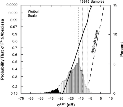
FIGURE 5.14 A measured VHF clutter histogram and cumulative distribution for a pure forest patch (WM/4/2) at Wachusett Mt., Mass.

FIGURE 5.15 A measured X-band clutter histogram and cumulative distribution for a pure farmland patch (WO 7/1) at Wolseley, Sask.
The two histograms of Figures 5.14 and 5.15 are both quite well behaved but are of extremely different shapes. In both figures, the measured cumulative distribution is plotted against a Weibull probability scale to the left. Both cumulatives are quite linear as plotted against this scale and hence are very well modeled as Weibull distributions [their coefficients of determination are 0.9994 and 0.9996, respectively; see Equation (2.B.30)]. The shape parameter aw of the Weibull distribution for the pure forest patch in Figure 5.14 is of value 1.7; it may be compared with the slope of the Rayleigh distribution of aw = 1 also shown in the figure. Although aw = 1.7 is significantly removed from aw = 1.0 (i.e., the distribution of Figure 5.14 is not a Rayleigh distribution, compare its sd/mean and mean/median numbers of 2.5 and 4.6 dB with Rayleigh values of 0 and 1.6 dB; see Table 5.12), still the distribution of Figure 5.14 approaches Rayleigh about as closely as routinely occurs in the Phase One measurements. The reasons that the pure forest distribution of Figure 5.14 approaches Rayleigh are: (1) the forested land cover (which constitutes a relatively homogeneous scattering medium compared with farmland), (2) the relatively large cell sizes resulting from the 13° VHF azimuth beamwidth, and (3) the high depression angle (i.e., 6°) at which the measurement was obtained.
In contrast, the pure farmland distribution of Figure 5.15 is very spread out, with a shape parameter of aw = 4.7. This value of aw is about as high as routinely occurs in the Phase One data. The reasons that this distribution is of such high spread are: (1) it is discrete-dominated farmland, (2) it is of high spatial resolution (i.e., 15-m range resolution and 1° azimuth beamwidth), and (3) it is of relatively low depression angle (i.e., 0.7°). The reason the cumulative tails off at its left end in Figure 5.15 is because it is being drawn down by the noise contamination (shown in black) at the low end of the histogram. As discussed previously, such noise contamination when included properly in computations does not adversely affect the moments, or the cumulative in the region to the right of the contamination.
The two pure clutter patch measurements shown in Figures 5.14 and 5.15 may be compared with the two mixed-terrain measurements shown previously in Chapter 5 in Figures 5.2 and 5.3. Both pairs of measurements exhibit extremely wide ranges in clutter strength (i.e., > 5 and > 8 orders of magnitude in Figures 5.14 and 5.15, respectively); and both pairs are reasonably well modeled as Weibull distributions over these wide ranges. The pure forest histogram of Figure 5.14 approaches Rayleigh more closely than the mixed forest/agricultural histogram of Figure 5.2, and the pure farmland histogram of Figure 5.15 is of greater spread (i.e., further from Rayleigh) than the mixed farmland/forest histogram of Figure 5.3. As discussed elsewhere in this book, every clutter patch measurement is different. Rather than rely on individual measurements such as are shown in Figures 5.14 and 5.15 for pure-terrain modeling information, what is done subsequently in Section 5.4 (as heretofore in Section 5.3) is to assemble large numbers of like-classified pure-terrain patch measurements, and to seek general modeling trends in the medianized results of ![]() and aw over many measurements.
and aw over many measurements.
Uncertain Outliers. There are generally large numbers of clutter patches within each terrain type/depression angle/radar parameter category. In processing clutter measurement results involving large numbers of patches, criteria are automatically applied ensuring that each patch measurement is valid (e.g., precluding excessive amounts of noise and/or saturation contamination, requiring close upper and lower mean bounds, etc.). Beyond this, it is generally not practicable to individually examine the measurement results from each clutter patch within a category. When the number of patch measurements within a category is large, occasional borderline measurements which, if individually examined, might be deleted as inappropriate to that category generally have negligible effect on the resulting median value of ![]() or aw for that category.
or aw for that category.
When the number of patch measurements within a category is small and the median value appears out-of-line with the expected trend, an open plot symbol is used to indicate that the value is an uncertain outlier (see Section 5.2.3.3). Since the number of patch measurements associated with uncertain outliers is small, it becomes practicable to occasionally examine individual patch measurements in such cases to determine if there is a discernible reason for the out-of-trend result. Some examples of such individual examination of uncertain outlier results are provided in following subsections addressing urban, agricultural, and forest terrain types.
5.4.1 URBAN OR BUILT-UP TERRAIN
By urban terrain is meant any kind of built-up land predominantly covered with structures, from high-rise centers of large cities (e.g., Calgary, Winnipeg, Scranton) to small country villages and remote military bases or industrial complexes. The urban clutter modeling information of Section 5.4.1 is based on 1,282 measured clutter histograms from 64 pure urban clutter patches at 18 measurement sites. Table 5.13 shows how these numbers of urban clutter patches and measured clutter histograms break down by depression angle in five regimes of depression angle. All of these urban clutter measurements were in pure low-relief terrain of terrain slope < 2°.
TABLE 5.13
Numbers of Terrain Patches and Measured Clutter Histograms for Urban or Built-up Terrain, by Depression Anglea,b,c

aA single (primary) classifier only is sufficient to describe these patches.
bA terrain patch is a land surface macroregion usually several kms on a side (median patch area = 12.62 km2).
cA measured clutter histogram contains all of the temporal (pulse by pulse) and spatial (resolution cell by resolution cell) clutter samples obtained in a given measurement of a terrain patch. A terrain patch was usually measured many times (nominally 20) as RF frequency (5), polarization (2), and range resolution (2) were varied over the Phase One radar parameter matrix.
Trends in ![]() Table 5.14 presents mean clutter strength
Table 5.14 presents mean clutter strength ![]() for urban terrain by frequency band, polarization, and depression angle, and includes the number of measurements upon which each value of
for urban terrain by frequency band, polarization, and depression angle, and includes the number of measurements upon which each value of ![]() is based. The
is based. The ![]() data of Table 5.14 are plotted in Figure 5.16. In Figure 5.16, consider first the
data of Table 5.14 are plotted in Figure 5.16. In Figure 5.16, consider first the ![]() data at positive depression angle (i.e., cyan, dark blue, purple, magenta). These data show two trends with frequency. The cyan and dark blue, low depression angle data (i.e., 0° to 0.25° and 0.25° to 0.75°) show increasing
data at positive depression angle (i.e., cyan, dark blue, purple, magenta). These data show two trends with frequency. The cyan and dark blue, low depression angle data (i.e., 0° to 0.25° and 0.25° to 0.75°) show increasing ![]() with increasing frequency, from about −35 dB at VHF to about −16 dB at X-band. The purple and magenta, high depression angle data (i.e., 0.75° to 1.5° and 1.5° to 4°) show frequency invariance of
with increasing frequency, from about −35 dB at VHF to about −16 dB at X-band. The purple and magenta, high depression angle data (i.e., 0.75° to 1.5° and 1.5° to 4°) show frequency invariance of ![]() largely within the −15 to −20 dB range in all five frequency bands. The low depression angle data were almost entirely measured at low site elevations over low-relief open terrain supportive of multipath; thus the lower
largely within the −15 to −20 dB range in all five frequency bands. The low depression angle data were almost entirely measured at low site elevations over low-relief open terrain supportive of multipath; thus the lower ![]() levels in the lower bands at low depression angles are due to multipath loss entering clutter strength σ°F4 through the propagation factor F. The high depression angle data were largely measured at higher site elevations in forested terrain not conducive to multipath; hence these high depression angle
levels in the lower bands at low depression angles are due to multipath loss entering clutter strength σ°F4 through the propagation factor F. The high depression angle data were largely measured at higher site elevations in forested terrain not conducive to multipath; hence these high depression angle ![]() data are more indicative of intrinsic σ° levels. At X-band, both high and low depression angle data indicate
data are more indicative of intrinsic σ° levels. At X-band, both high and low depression angle data indicate ![]() at vertical polarization to be significantly stronger (viz., by 3 to 6 dB) than at horizontal polarization. This clear-cut difference with polarization at X-band is much less evident in the lower bands.
at vertical polarization to be significantly stronger (viz., by 3 to 6 dB) than at horizontal polarization. This clear-cut difference with polarization at X-band is much less evident in the lower bands.
TABLE 5.14
Mean Clutter Strength ![]() and Number of Measurements for Urban or Built-up Terrain, by Frequency Band, Polarization, and Depression Anglea
and Number of Measurements for Urban or Built-up Terrain, by Frequency Band, Polarization, and Depression Anglea


aTable 5.13 defines the population of terrain patches upon which these data are based.

Uncertain Outliers. Next, in Figure 5.16, consider the ![]() data at negative depression angle (dark green, 0° to −0.25°). These data come from seven clutter patches at three sites. These dark green, negative depression angle
data at negative depression angle (dark green, 0° to −0.25°). These data come from seven clutter patches at three sites. These dark green, negative depression angle ![]() data are considerably weaker in all bands than the corresponding
data are considerably weaker in all bands than the corresponding ![]() data at positive depression angles. The reason for the low levels in the dark green, negative depression angle
data at positive depression angles. The reason for the low levels in the dark green, negative depression angle ![]() data in Figure 5.16 is that all seven clutter patches contributing to the dark green data were measured with positive effective radar height h, but at long ranges r of 20 to 40 km which were beyond the imaginary28 spherical earth horizon r’ in all cases. Thus the negative depression angle is the result of geometry on the spherical earth, not the result of negative effective radar height (see Appendix 2.C). This is not to suggest that the negative depression angle that results at long ranges r > r’ on the spherical earth with h > 0 is any less real than that resulting from h < 0 at short ranges r < r’—but that considerable propagation loss occurs over the long intervening ranges, which accounts for the low levels of the dark green, negative depression angle
data in Figure 5.16 is that all seven clutter patches contributing to the dark green data were measured with positive effective radar height h, but at long ranges r of 20 to 40 km which were beyond the imaginary28 spherical earth horizon r’ in all cases. Thus the negative depression angle is the result of geometry on the spherical earth, not the result of negative effective radar height (see Appendix 2.C). This is not to suggest that the negative depression angle that results at long ranges r > r’ on the spherical earth with h > 0 is any less real than that resulting from h < 0 at short ranges r < r’—but that considerable propagation loss occurs over the long intervening ranges, which accounts for the low levels of the dark green, negative depression angle ![]() data in Figure 5.16. Such propagation loss would not exist in short range, negative depression angle urban
data in Figure 5.16. Such propagation loss would not exist in short range, negative depression angle urban ![]() data in h < 0 situations. Therefore, the dark green, negative depression angle
data in h < 0 situations. Therefore, the dark green, negative depression angle ![]() data in Figure 5.16 are plotted as open symbols to indicate that urban clutter that might be measured from steep slopes at higher elevations than the radar antenna (N.B., no such measurements exist in the Phase One database) should not be assumed to be generally weaker than urban clutter at positive depression angle.
data in Figure 5.16 are plotted as open symbols to indicate that urban clutter that might be measured from steep slopes at higher elevations than the radar antenna (N.B., no such measurements exist in the Phase One database) should not be assumed to be generally weaker than urban clutter at positive depression angle.
Strong Urban (and Mountain) Clutter. The high depression angle, urban ![]() data in Table 5.14 and Figure 5.16 (plotted as purple and magenta) represent very strong values of mean land clutter strength. Among the eight specific terrain types discussed in Section 5.4, mountain terrain also provides strong values of
data in Table 5.14 and Figure 5.16 (plotted as purple and magenta) represent very strong values of mean land clutter strength. Among the eight specific terrain types discussed in Section 5.4, mountain terrain also provides strong values of ![]() . The purple and magenta, urban
. The purple and magenta, urban ![]() data of Figure 5.16 are stronger than the mountain
data of Figure 5.16 are stronger than the mountain ![]() data of Section 5.4.8 at X- and S-band, approximately equal to (or slightly stronger than) the strongest values of mountain
data of Section 5.4.8 at X- and S-band, approximately equal to (or slightly stronger than) the strongest values of mountain ![]() at L-band, and weaker than the strongest values of mountain
at L-band, and weaker than the strongest values of mountain ![]() at UHF and VHF—slightly weaker at UHF and much weaker at VHF. That is, urban clutter is generally strongest in the high bands, and mountain clutter is generally strongest in the low bands. In each of the five Phase One frequency bands, either urban or mountain terrain provides the maximum value of
at UHF and VHF—slightly weaker at UHF and much weaker at VHF. That is, urban clutter is generally strongest in the high bands, and mountain clutter is generally strongest in the low bands. In each of the five Phase One frequency bands, either urban or mountain terrain provides the maximum value of ![]() among the eight specific terrain types of Section 5.4. By frequency band, these five maximum values of
among the eight specific terrain types of Section 5.4. By frequency band, these five maximum values of ![]() are: at VHF, −5.8 dB (mountains); at UHF, −12.4 dB (mountains); at L-band, −14.9 dB (urban); at S-band, −15.4 dB (urban); and at X-band, −12.9 dB (urban).
are: at VHF, −5.8 dB (mountains); at UHF, −12.4 dB (mountains); at L-band, −14.9 dB (urban); at S-band, −15.4 dB (urban); and at X-band, −12.9 dB (urban).
The urban ![]() values of Table 5.14 and Figure 5.16 represent median levels of mean clutter strength from groups of like-classified clutter patches—individual patches can be stronger. In each of the five Phase One frequency bands, the strongest mean clutter strength from a pure urban clutter patch was: at VHF, 9.8 dB; at UHF, 0.3 dB; at L-band, 0.0 dB; at S-band, −5.8 dB; and at X-band, −0.5 dB.
values of Table 5.14 and Figure 5.16 represent median levels of mean clutter strength from groups of like-classified clutter patches—individual patches can be stronger. In each of the five Phase One frequency bands, the strongest mean clutter strength from a pure urban clutter patch was: at VHF, 9.8 dB; at UHF, 0.3 dB; at L-band, 0.0 dB; at S-band, −5.8 dB; and at X-band, −0.5 dB.
The urban ![]() data of Table 5.14 and Figure 5.16 indicate a strong depression angle dependence in the lower bands. As discussed previously, this effect is largely due to multipath loss in the results at low depression angles. However, intrinsic σ° at VHF may also increase with depression angle in urban terrain. At one site, Cochrane, five clutter histograms at VHF were measured from one urban clutter patch at the high depression angle of 7.8° (these data are not included in Figure 5.16). The range of mean strengths in these five histograms was 4.0 to 6.1 dB, considerably stronger than the −16.3 to −20.6 dB VHF levels in the 0.75° to 4° depression angle range in Table 5.14 and Figure 5.16. Besides the high depression angle, another factor that contributed to these high VHF urban clutter levels at Cochrane is that the terrain of the patch was of mixed landform—generally level, but with a moderately steep component along the bank of a river dissecting the patch. In the higher bands, there is little indication of depression angle dependence in the urban
data of Table 5.14 and Figure 5.16 indicate a strong depression angle dependence in the lower bands. As discussed previously, this effect is largely due to multipath loss in the results at low depression angles. However, intrinsic σ° at VHF may also increase with depression angle in urban terrain. At one site, Cochrane, five clutter histograms at VHF were measured from one urban clutter patch at the high depression angle of 7.8° (these data are not included in Figure 5.16). The range of mean strengths in these five histograms was 4.0 to 6.1 dB, considerably stronger than the −16.3 to −20.6 dB VHF levels in the 0.75° to 4° depression angle range in Table 5.14 and Figure 5.16. Besides the high depression angle, another factor that contributed to these high VHF urban clutter levels at Cochrane is that the terrain of the patch was of mixed landform—generally level, but with a moderately steep component along the bank of a river dissecting the patch. In the higher bands, there is little indication of depression angle dependence in the urban ![]() data of Table 5.14 and Figure 5.16.
data of Table 5.14 and Figure 5.16.
Shape Parameter aw. Table 5.15 presents the Weibull shape parameter aw and ratios of standard deviation-to-mean and mean-to-median for clutter amplitude distributions in low-relief urban terrain by depression angle and radar spatial resolution. The statistical populations underlying the data of Table 5.15 are shown in Table 5.13. In Table 5.15 and other similar tables in Chapter 5, aw is calculated two ways: (1) from the ratio of standard deviation-to-mean and (2) from the mean-to-median ratio. Many of the corresponding aw numbers resulting from these two methods of calculation are relatively close in Table 5.15; however, several of these corresponding aw numbers in Table 5.15 are not close, indicating that urban clutter can in some situations be less well approximated as Weibull distributed than other types of land clutter.
TABLE 5.15
Shape Parameter aw and Ratios of Standard Deviation-to-Mean (SD/Mean) and Mean-to-Median for Urban or Built-up Terrain, by Spatial Resolution A and Depression Angle*


aFootnoted values apply at A = 105 m2, not 106 m2.
bFootnoted values apply at A = 104 m2, not 103 m2.
*Table 5.13 defines the population of terrain patches and measurements upon which these data are based.
The major parametric variation of aw in Table 5.15 is with radar spatial resolution. In every case, aw is much greater at 103 m2 resolution than at 106 m2 resolution. At low depression angle (i.e., 0° to 0.25°), Table 5.15 indicates that spreads in urban terrain, although high, are not unusually high compared to many other terrain types. However, most terrain types show significantly smaller spreads at high depression angle. In contrast, Table 5.15 indicates that in urban terrain at high spatial resolution (i.e., A = 103 m2), spreads remain high at high depression angle.
Each pair of aw numbers in Table 5.15 comes from a scatter plot of spread vs spatial resolution. The standard deviation-to-mean scatter plot for the 0° to 0.25° depression angle regime in Table 5.15 is shown in Figure 5.17. The main trend in Figure 5.17 is decreasing spread with decreasing resolution. In the wide pulse data in the lower frequency bands, spreads in the first range interval are less than in the second and third range intervals, contrary to expectation. This tendency is not borne out in the narrow pulse data.

5.4.2 AGRICULTURAL TERRAIN
As in urban terrain, the dominant clutter sources in agricultural terrain are often specific discrete vertical objects associated with man’s use of the land. Clutter strengths can depend quite specifically on what particular discretes exist and how they are distributed over a clutter patch. Unlike urban terrain, however, in agricultural terrain the occasional (e.g., 20% incidence) strong isolated discrete cells occur in a weakly scattering background. Many of the strong cells occur in definite, culturally determined, spatial patterns. Thus farmland clutter is quite a different, more heterogeneous, statistical random process than clutter from terrain with more natural land cover—for example, forest. Furthermore, multipath exists in many of the Phase One farmland clutter measurements to cause additional specific variations in clutter strength through the propagation factor, depending on the specific variations of terrain elevation involved (see Section 3.4.1.4). As a result of this multifold specificity affecting clutter strengths in agricultural terrain, more measurements are required to establish generality in agricultural terrain than in more homogeneous terrain such as forest. As shown in Table 5.16, the farmland clutter modeling information of Section 5.4.2 is based on 10,357 measured clutter histograms from 525 clutter patches. These results come from 30 measurement sites. These are the largest numbers of measurements, patches, and sites among the eight specific terrain types of Section 5.4. In what follows, multifrequency clutter coefficients are presented for agricultural terrain in three regimes of relief: (1) high-relief, (2) low-relief, and (3) level.
TABLE 5.16
Numbers of Terrain Patches and Measured Clutter Histograms for Agricultural Terrain, by Relief and Depression Anglea,b,c

aA single (primary) classifier only is sufficient to describe these patches.
bA terrain patch is a land surface macroregion usually several kms on a side (median patch area = 12.62 km2).
cA measured clutter histogram contains all of the temporal (pulse by pulse) and spatial (resolution cell by resolution cell) clutter samples obtained in a given measurement of a terrain patch. A terrain patch was usually measured many times (nominally 20) as RF frequency (5), polarization (2), and range resolution (2) were varied over the Phase One radar parameter matrix.
Seasonal Effects. Agricultural terrain is primarily cropland. The status of the crops in the fields depends upon season. During summer season, changes from before to after harvest occur. During winter season, cropland fields are generally fallow or stubble, often with various degrees of snow cover. Approximately 45% of the clutter measurements occurred in winter season. Perhaps surprisingly, farmland clutter is not highly sensitive to the changing seasonal status of the fields because it is dominated by isolated discrete sources that exist independent of season. The field surfaces contribute to low-level background clutter whatever their seasonal status. Seasonal variations in the land clutter measurements, including agricultural terrain, are discussed in Chapters 2 and 3. Since general seasonal effects in land clutter are small, the clutter modeling information presented in Chapter 5 does not include season as a parametric dimension.
5.4.2.1 HIGH-RELIEF AGRICULTURAL TERRAIN
Trends in ![]() . Table 5.17 presents mean clutter strength for high-relief agricultural terrain by frequency band, polarization, and depression angle and includes the number of measurements upon which each value of
. Table 5.17 presents mean clutter strength for high-relief agricultural terrain by frequency band, polarization, and depression angle and includes the number of measurements upon which each value of ![]() is based. Relatively little Phase One measurement data exists for high-relief agricultural terrain—just 250 measured clutter histograms from 20 clutter patches at eight measurement sites. The primary reason for this sparsity of data is that little high-relief farmland exists; farm machinery cannot easily access high-relief terrain.
is based. Relatively little Phase One measurement data exists for high-relief agricultural terrain—just 250 measured clutter histograms from 20 clutter patches at eight measurement sites. The primary reason for this sparsity of data is that little high-relief farmland exists; farm machinery cannot easily access high-relief terrain.
TABLE 5.17
Mean Clutter Strength ![]() and Number of Measurements for High-Relief Agricultural Terrain, by Frequency Band, Polarization, and Depression Anglea
and Number of Measurements for High-Relief Agricultural Terrain, by Frequency Band, Polarization, and Depression Anglea


aTable 5.16 defines the population of terrain patches upon which these data are based.
The ![]() data of Table 5.17 are plotted in Figure 5.18. Except for the uncertain outliers plotted as open symbols, the data of Figure 5.18 lie largely in the −29- to −36-dB range without major trends with frequency or depression angle. At first consideration, the cluster of L-band results appears 3 or 4 dB stronger than the other bands; however, the more reliable cyan (0° to 1°) results do not show stronger
data of Table 5.17 are plotted in Figure 5.18. Except for the uncertain outliers plotted as open symbols, the data of Figure 5.18 lie largely in the −29- to −36-dB range without major trends with frequency or depression angle. At first consideration, the cluster of L-band results appears 3 or 4 dB stronger than the other bands; however, the more reliable cyan (0° to 1°) results do not show stronger ![]() at L-band. In these results,
at L-band. In these results, ![]() at vertical polarization is usually several decibels stronger than at horizontal polarization.
at vertical polarization is usually several decibels stronger than at horizontal polarization.

Uncertain Outliers. Now consider the uncertain outliers in the ![]() results for high-relief agricultural terrain of Table 5.17. These uncertain results are plotted as open plot symbols in Figure 5.18. Within these uncertain outlier results in high-relief agricultural terrain, three particular clutter patch measurements are discussed. Two of these patch measurements involve borderline-high incidences of trees occurring within patches classified as pure farmland terrain causing stronger than expected outlier values of
results for high-relief agricultural terrain of Table 5.17. These uncertain results are plotted as open plot symbols in Figure 5.18. Within these uncertain outlier results in high-relief agricultural terrain, three particular clutter patch measurements are discussed. Two of these patch measurements involve borderline-high incidences of trees occurring within patches classified as pure farmland terrain causing stronger than expected outlier values of ![]() ; and one patch measurement involves a terrain inclination away from the radar causing a weaker than expected outlier value of
; and one patch measurement involves a terrain inclination away from the radar causing a weaker than expected outlier value of ![]() .
.
First consider the very strong, green (0° to −1°) results at VHF in Figure 5.18. These results are dominated by one strong clutter patch, viz., patch 37 at the Penhold measurement site in Alberta. This patch is classified as pure farmland, although with ∼10% tree cover. These patch 37 ![]() results agree very closely with corresponding results (not shown here) at VHF for high-relief mixed terrain classified as open/forest, these latter results being based on a large number of measurements. Thus it would appear that patch 37 at Penhold may have been more appropriately classified as mixed terrain with a secondary component of forest. Misclassification of occasional single patches is usually of little consequence in the general (i.e., medianized) results of Chapter 5 that are more typically based on measurements from many patches.
results agree very closely with corresponding results (not shown here) at VHF for high-relief mixed terrain classified as open/forest, these latter results being based on a large number of measurements. Thus it would appear that patch 37 at Penhold may have been more appropriately classified as mixed terrain with a secondary component of forest. Misclassification of occasional single patches is usually of little consequence in the general (i.e., medianized) results of Chapter 5 that are more typically based on measurements from many patches.
Next, consider the relatively strong, purple (2° to 4°) results at UHF in Figure 5.18. These results are based on measurements from one clutter patch, viz., patch 30 at the Polonia measurement site in Manitoba. Again, this patch is classified as pure farmland with ∼10% tree cover. Comparison with other results indicates that the clutter from patch 30 at Polonia was also very likely dominated by trees. That is, patch 30 at Polonia may also have been more appropriately classified as mixed open/forest. Most farmland has some small incidence of occurrence of trees. The percentage incidence at which trees begin to dominate the backscatter from farmland landscapes can be quite low. The results from these two patches show the importance in clutter prediction of accurately depicting the relative proportion of trees on generally open landscapes.
Finally, consider the relatively weak, dark blue (1° to 2°) results at VHF, S-, and X-band in Figure 5.18. These results are based almost entirely on three clutter patches, and, at S- and X-bands, on just two clutter patches. One of these patches, viz., patch 12 at the Magrath measurement site in Alberta, was relatively weak in all bands. Patch 12 was at close range (1.2 to 2.2 km) on the side of the slope at the top of which the Phase One radar was situated, and as a result may be weak due to its outward inclination and/or due to it being borderline-shadowed by intervening higher terrain (brow-of-hill effect; see Appendix 4.B). More measurements were made from patch 12 than the other contributing patches in the dark blue (1° to 2°) results in Figure 5.18 at VHF, S-, and X-band—hence the median result from the set is low in these bands. In contrast, more measurements were made from the other two contributing patches than from patch 12 at UHF and L-band—hence the median results from these sets are higher and in line with the data from the other depression angle regimes in Figure 5.18. It is evident from such considerations that caution must be exercised in using any Chapter 5 open-symbol results based on sparse data.
Shape Parameter aw. Table 5.18 presents the Weibull shape parameter aw and ratios of standard deviation-to-mean and mean-to-median for clutter amplitude distributions in high-relief agricultural terrain by depression angle and radar spatial resolution. The statistical populations underlying the data of Table 5.18 are shown in Table 5.16. Table 5.18 shows that very large values of spread occur in spatial clutter amplitude distributions at low angles and high resolution in high-relief agricultural terrain. In every case, aw is greater at 103 m2 resolution than at 106 (or 105) m2 resolution. At the higher resolution of 103 m2, aw also strongly depends on depression angle. In high-relief agricultural terrain, aw at high resolution decreases strongly from large values at grazing incidence (i.e., 0° to 1°) to much smaller values at higher angles (e.g., 2° to 4°). Therefore, modeling of clutter from high-relief agricultural terrain must be done in narrow regimes of depression angle to accommodate this strong trend of decreasing spread in clutter amplitude distributions with increasing angle of illumination, even though mean clutter strengths in high-relief agricultural terrain are relatively insensitive to angle of illumination.
TABLE 5.18
Shape Parameter aw and Ratios of Standard Deviation-to-Mean (SD/Mean) and Mean-to-Median for High-Relief Agricultural Terrain, by Spatial Resolution A and Depression Angle*


aFootnoted values apply at A = 105 m2, not 106 m2.
*Table 5.16 defines the population of terrain patches and measurements upon which these data are based.
Each pair of aw numbers in Table 5.18 comes from a scatter plot of spread vs spatial resolution. The standard deviation-to-mean scatter plot for the 1° to 2° depression angle regime in Table 5.18 is shown in Figure 5.19. The data in Figure 5.19 show a strong trend of decreasing spread with decreasing resolution (i.e., increasing A). Note that all of the results in Figure 5.19 happen to come from the first range interval, 1 to 11.3 km. As a result, it is easier to follow the variations with frequency and pulse length in this figure than in many of the similar scatter plots in Chapter 5. Further note that although the measured data extend only to A ≅ 105 m 2 in Figure 5.19, it is reasonable to extend the regression line to A = 106 m2; indeed, this was done to provide the sd/mean based results at A = 106 m2 for the 1° to 2° depression angle interval in Table 5.18. However, for the corresponding mean/median scatter plot, it was not reasonable to extend the regression line to A = 106 m2; hence the mean/median based results are shown at A = 105 m2, not A = 106 m2, for the 1° to 2° depression angle regime in Table 5.18.

5.4.2.2 LOW-RELIEF AGRICULTURAL TERRAIN
Trends in ![]() . Table 5.19 presents mean clutter strength
. Table 5.19 presents mean clutter strength ![]() for low-relief agricultural terrain by frequency band, polarization, and depression angle and includes the number of measurements upon which each value of
for low-relief agricultural terrain by frequency band, polarization, and depression angle and includes the number of measurements upon which each value of ![]() is based. These results are based on a very large amount of Phase One measurement data—10,107 measured clutter histograms from 505 clutter patches; see Table 5.16. These measurements come from 30 sites.
is based. These results are based on a very large amount of Phase One measurement data—10,107 measured clutter histograms from 505 clutter patches; see Table 5.16. These measurements come from 30 sites.
TABLE 5.19
Mean Clutter Strength ![]() and Number of Measurements for Low-Relief Agricultural Terrain, by Frequency Band, Polarization, and Depression Anglea
and Number of Measurements for Low-Relief Agricultural Terrain, by Frequency Band, Polarization, and Depression Anglea


aTable 5.16 defines the population of terrain patches upon which these data are based.
The ![]() data of Table 5.19 are plotted in Figure 5.20. The main parametric trend observed in Figure 5.20 is that
data of Table 5.19 are plotted in Figure 5.20. The main parametric trend observed in Figure 5.20 is that ![]() increases significantly—by about 10 dB—with increasing frequency, VHF through L-band, then levels off, L-band through X-band. Weaker values of
increases significantly—by about 10 dB—with increasing frequency, VHF through L-band, then levels off, L-band through X-band. Weaker values of ![]() at VHF and UHF are due to multipath loss from forward reflections on generally open, low-relief, agricultural terrain. At the lower frequencies, the multipath lobes on the elevation pattern are broad, and returns from clutter sources are typically received at reduced gain well on the underside of the first multipath lobe. At the higher frequencies, the multipath lobes are narrower and clutter sources tend to be more fully illuminated. The details of the multipath depend on the terrain between the clutter patch and the radar. Some patches will experience more multipath loss and some less (see Section 3.4.1.4). Figure 5.20 shows medianized results from many measurements in generally low-relief agricultural terrain.
at VHF and UHF are due to multipath loss from forward reflections on generally open, low-relief, agricultural terrain. At the lower frequencies, the multipath lobes on the elevation pattern are broad, and returns from clutter sources are typically received at reduced gain well on the underside of the first multipath lobe. At the higher frequencies, the multipath lobes are narrower and clutter sources tend to be more fully illuminated. The details of the multipath depend on the terrain between the clutter patch and the radar. Some patches will experience more multipath loss and some less (see Section 3.4.1.4). Figure 5.20 shows medianized results from many measurements in generally low-relief agricultural terrain.

The ![]() results of Figure 5.20 show little variation with depression angle. The results at X-band form a very tight cluster. The results from L-band through X-band are remarkably invariant with both frequency and depression angle, all largely in the −29 dB to −33 dB range. At first consideration, the results at UHF appear to show increasing
results of Figure 5.20 show little variation with depression angle. The results at X-band form a very tight cluster. The results from L-band through X-band are remarkably invariant with both frequency and depression angle, all largely in the −29 dB to −33 dB range. At first consideration, the results at UHF appear to show increasing ![]() with increasing positive depression angle. However, further consideration of these UHF data reveals that, in the cyan, 0° to 0.25° results, large multipath loss exists, as large as that which exists in the cyan results at VHF, but in the dark blue, purple, and magenta, higher depression angle UHF results, the multipath loss is less and little or no variation of
with increasing positive depression angle. However, further consideration of these UHF data reveals that, in the cyan, 0° to 0.25° results, large multipath loss exists, as large as that which exists in the cyan results at VHF, but in the dark blue, purple, and magenta, higher depression angle UHF results, the multipath loss is less and little or no variation of ![]() occurs with depression angle in these higher angle results. Note that in the dark blue, 0.25° to 0.75° results in Figure 5.20,
occurs with depression angle in these higher angle results. Note that in the dark blue, 0.25° to 0.75° results in Figure 5.20, ![]() at S-band is approximately equal to
at S-band is approximately equal to ![]() at L-band and X-band, but with increasing depression angle, purple, 0.75° to 1.5°, through magenta, 1.5° to 4°,
at L-band and X-band, but with increasing depression angle, purple, 0.75° to 1.5°, through magenta, 1.5° to 4°, ![]() at S-band increasingly dips below
at S-band increasingly dips below ![]() at L-band and X-band. A more significant S-band dip at high depression angle was discussed in the low-relief general mixed rural results of Figure 5.10.
at L-band and X-band. A more significant S-band dip at high depression angle was discussed in the low-relief general mixed rural results of Figure 5.10.
At X-band in Figure 5.20, ![]() is one or two dB stronger than
is one or two dB stronger than ![]() in every depression angle regime. This slight polarization bias continues to be largely true at S-band but is less evident at the lower frequencies, and at VHF is reversed such that
in every depression angle regime. This slight polarization bias continues to be largely true at S-band but is less evident at the lower frequencies, and at VHF is reversed such that ![]() is generally slightly stronger than
is generally slightly stronger than ![]() .
.
Uncertain Outliers. Now consider the uncertain outliers in ![]() results for low-relief agricultural terrain which are plotted as open plot symbols in Figure 5.20. First consider the light green, −0.25° to −0.75° results. Table 5.19 shows that these results are based on significantly fewer measurements than the other depression angle regimes. At VHF these light green results show a very significant difference with polarization, with
results for low-relief agricultural terrain which are plotted as open plot symbols in Figure 5.20. First consider the light green, −0.25° to −0.75° results. Table 5.19 shows that these results are based on significantly fewer measurements than the other depression angle regimes. At VHF these light green results show a very significant difference with polarization, with ![]() stronger than
stronger than ![]() by 13 dB. At horizontal polarization, the light green result at VHF comes from five measurements, four from the Altona site and one from a very weak clutter patch at the Neepawa site. Thus at horizontal polarization, the median measurement is an Altona measurement. At vertical polarization, however, the light green result at VHF comes from only two measurements, both from the weak Neepawa patch. Thus at vertical polarization, the median measurement is an atypically weak Neepawa measurement. At UHF the light green, −0.25° to −0.75° results in Figure 5.20 no longer show a polarization difference, but remain dependent on relatively few samples, and are significantly weaker than the dark green, 0° to −0.25° results. One reason that the light green, −0.25° to −0.75°
by 13 dB. At horizontal polarization, the light green result at VHF comes from five measurements, four from the Altona site and one from a very weak clutter patch at the Neepawa site. Thus at horizontal polarization, the median measurement is an Altona measurement. At vertical polarization, however, the light green result at VHF comes from only two measurements, both from the weak Neepawa patch. Thus at vertical polarization, the median measurement is an atypically weak Neepawa measurement. At UHF the light green, −0.25° to −0.75° results in Figure 5.20 no longer show a polarization difference, but remain dependent on relatively few samples, and are significantly weaker than the dark green, 0° to −0.25° results. One reason that the light green, −0.25° to −0.75° ![]() results are relatively weak at UHF and, indeed, also relatively weak at S-band and X-band is that among the 15 clutter patches contributing to these results are three clutter patches that exist at long ranges, from 35 to 65 km. For these three patches, effective radar height is negative, on the order of several hundred feet. Even so, these three patches are at ranges nearly as great as (i.e., one patch) or significantly greater than (i.e., two patches) the quantity
results are relatively weak at UHF and, indeed, also relatively weak at S-band and X-band is that among the 15 clutter patches contributing to these results are three clutter patches that exist at long ranges, from 35 to 65 km. For these three patches, effective radar height is negative, on the order of several hundred feet. Even so, these three patches are at ranges nearly as great as (i.e., one patch) or significantly greater than (i.e., two patches) the quantity ![]() (see Appendix 2.C). Therefore, much of the negative depression angle to these three patches is caused by geometry on the spherical earth. These patches are weak because of diffraction loss due to propagation over the long ranges of intervening terrain at near grazing incidence. Similarly weak clutter occurring for long-range urban patches is discussed in Section 5.4.1.
(see Appendix 2.C). Therefore, much of the negative depression angle to these three patches is caused by geometry on the spherical earth. These patches are weak because of diffraction loss due to propagation over the long ranges of intervening terrain at near grazing incidence. Similarly weak clutter occurring for long-range urban patches is discussed in Section 5.4.1.
Now consider the magenta, 1.5° to 4° results in Figure 5.20. At S-band these magenta results show a significant dip of 5 to 6 dB below the magenta results at L-band and X-band. These magenta results also are based on fewer measurements than in the lower depression angle regimes in Figure 5.20. Among these measurements are those from one relatively weak clutter patch, viz., patch 31, at the Beiseker measurement site. Patch 31 was at close range (1.0 to 2.2 km) on the side of the long hill upon which the Phase One radar was situated at Beiseker and, therefore, may have been borderline-shadowed (brow-of-hill effect). Deleting the patch 31 measurements would significantly raise the magenta S-band results in Figure 5.20 but would have less effect at X-band. Thus the exaggerated S-band dip in the magenta results in Figure 5.20 may partially reflect a real effect, but in addition may be partially due to atypically weak S-band clutter from patch 31 at Beiseker.
Shape Parameter aw. Table 5.20 presents the Weibull shape parameter aw and ratios of standard deviation-to-mean and mean-to-median for clutter amplitude distributions in low-relief agricultural terrain by depression angle and radar spatial resolution. The statistical populations underlying the data of Table 5.20 are shown in Table 5.16. Table 5.20 shows that very large values of spread occur in spatial clutter amplitude distributions at low angles and high resolution in low-relief agricultural terrain. For example, at near grazing incidence (i.e., 0° to 0.25° depression angle) and at high resolution (i.e., A = 103 m2), ratios of mean-to-median and standard deviation-to-mean of 29.5 dB and 13.7 dB, respectively, indicate a very highly skewed distribution.
TABLE 5.20
Shape Parameter aw and Ratios of Standard Deviation-to-Mean (SD/Mean) and Mean-to-Median for Low-Relief Agricultural Terrain, by Spatial Resolution A and Depression Angle*


aFootnoted values apply at A = 105 m2, not 106 m2.
*Table 5.16 defines the population of terrain patches and measurements upon which these data are based.
The main parametric trend of aw in Table 5.20 is with radar spatial resolution. In every case, aw is greater at 103 m2 resolution that at 106 m2 resolution. However, at the higher resolution of 103 m2, aw also strongly depends on depression angle. That is, in low-relief agricultural terrain, although ![]() is largely invariant with depression angle, aw at high resolution decreases strongly from large values at grazing incidence (i.e., 0° to 0.25°) to much smaller values at higher angles. Consideration of Table 5.16 and comparison of Table 5.20 with Table 5.18 indicates that this trend in low-relief agricultural terrain is supported by a much larger population of measurements separated into more finely graduated depression angle regimes than the corresponding trend in high-relief agricultural terrain. Therefore, as in high-relief agricultural terrain, modeling of clutter in low-relief agricultural terrain must still be done in narrow regimes of depression angle to accommodate this strong trend of decreasing spread in clutter amplitude distributions with increasing angle of illumination, even though mean clutter strengths in low-relief agricultural terrain are relatively insensitive to angle of illumination.
is largely invariant with depression angle, aw at high resolution decreases strongly from large values at grazing incidence (i.e., 0° to 0.25°) to much smaller values at higher angles. Consideration of Table 5.16 and comparison of Table 5.20 with Table 5.18 indicates that this trend in low-relief agricultural terrain is supported by a much larger population of measurements separated into more finely graduated depression angle regimes than the corresponding trend in high-relief agricultural terrain. Therefore, as in high-relief agricultural terrain, modeling of clutter in low-relief agricultural terrain must still be done in narrow regimes of depression angle to accommodate this strong trend of decreasing spread in clutter amplitude distributions with increasing angle of illumination, even though mean clutter strengths in low-relief agricultural terrain are relatively insensitive to angle of illumination.
The reasons that depression angle affects spread (see Table 5.20) but not mean strength (see Figure 5.20 and Table 5.19) in clutter spatial amplitude distributions in low-relief farmland are as follows. In low-relief farmland, dominant clutter sources are large, discrete, vertical objects. At low angles strong returns are received from these discrete sources, but much (e.g., 75%) of the intervening terrain is either shadowed or provides very weak returns due to the illumination being at grazing incidence. As a result, in low-relief farmland at low depression angle clutter amplitude distributions have very large spread. As depression angle increases, the intervening terrain between strong discrete sources comes under stronger illumination. The weak returns from these regions rapidly increase, and as a result spreads in amplitude distributions rapidly decrease, as shown in Table 5.20. However, the strong returns from the discrete objects at the high ends of the distributions tend to be relatively independent of depression angle and continue to dominate their mean strengths, with the result that the mean strengths in low-relief farmland as shown in Table 5.19 and Figure 5.20 are largely independent of depression angle (cf. Chapter 2, Figure 2.47).
Each pair of aw numbers in Table 5.20 comes from a scatter plot of spread vs spatial resolution. The standard deviation-to-mean scatter plot for the 0° to 0.25° depression angle regime in Table 5.20 is shown in Figure 5.21. The data in Figure 5.21 show a very strong trend of decreasing spread with decreasing resolution (i.e., increasing A). There is a very large amount of measurement data underlying the scatter plot of Figure 5.21; see Table 5.16. In terms of plot symbols, Figure 5.21 is more highly populated than most similar scatter plots in Chapter 5, only missing three plot symbols, i.e., only missing narrow pulse data in the third range interval in the three high bands. Not only does the regression line in Figure 5.21 show a very strong trend whereby the ratio of standard deviation-to-mean rapidly drops from very high values—among the highest of any presented in Chapter 5—to very low values with increasing A, but in addition the plot symbols are for the most part tightly correlated to the regression line and show relatively little scatter away from this line.

FIGURE 5.21 Ratio of standard deviation-to-mean (SD/Mean) vs radar spatial resolution A for low-relief agricultural terrain with depression angle between 0.0 and 0.25 degrees.
Underlying Variability. In low-angle land clutter there is considerable patch-to-patch variability for any given specification of terrain type, relief, depression angle, and radar parameters. This is particularly true in low-relief agricultural terrain where specific influences of discrete sources and propagation prevail. For example, consider the results in the dark blue, 0.25° to 0.75° depression angle regime in Figure 5.20 and Table 5.19, which is the depression angle regime containing the largest number of measurements in low-relief agricultural terrain. In Figure 5.20, these dark blue results show a smooth trend of increasing ![]() with frequency, VHF to L-band, which levels off from L-band through X-band. Underlying this smooth general trend is considerable patch-to-patch variability. Within these dark blue data, the maximum and minimum values of mean clutter strength within the set of contributing like-classified measurements26 in each frequency band are as follows: at VHF, −6.1 and −72.2 dB; at UHF, −10.7 and −74.4 dB; at L-band, −7.8 and −75.7 dB; at S-band, −10.9 and −73.5 dB; and at X-band, −15.1 and −50.0 dB. The standard deviation of the decibel values of mean clutter strength as a measure of spread in each frequency band is: at VHF, 12.7 dB; at UHF, 11.0 dB; at L-band, 8.8 dB; at S-band, 7.2 dB; and at X-band, 4.8 dB. Thus significantly decreasing patch-to-patch variability in mean clutter strength occurs with increasing frequency VHF through X-band in low-relief agricultural terrain (cf. corresponding discussion based on repeat sector data in Chapter 3 at the end of Section 3.7.3). The principal reason for this decreasing variability with increasing frequency is that propagation influences diminish with increasing frequency. Such underlying patch-to-patch variability makes clear why selected individual measurements historically did not lead to a very clear overall picture of the general characteristics of low-angle land clutter. As indicated here, a large amount of measurement data is required to find general trends.
with frequency, VHF to L-band, which levels off from L-band through X-band. Underlying this smooth general trend is considerable patch-to-patch variability. Within these dark blue data, the maximum and minimum values of mean clutter strength within the set of contributing like-classified measurements26 in each frequency band are as follows: at VHF, −6.1 and −72.2 dB; at UHF, −10.7 and −74.4 dB; at L-band, −7.8 and −75.7 dB; at S-band, −10.9 and −73.5 dB; and at X-band, −15.1 and −50.0 dB. The standard deviation of the decibel values of mean clutter strength as a measure of spread in each frequency band is: at VHF, 12.7 dB; at UHF, 11.0 dB; at L-band, 8.8 dB; at S-band, 7.2 dB; and at X-band, 4.8 dB. Thus significantly decreasing patch-to-patch variability in mean clutter strength occurs with increasing frequency VHF through X-band in low-relief agricultural terrain (cf. corresponding discussion based on repeat sector data in Chapter 3 at the end of Section 3.7.3). The principal reason for this decreasing variability with increasing frequency is that propagation influences diminish with increasing frequency. Such underlying patch-to-patch variability makes clear why selected individual measurements historically did not lead to a very clear overall picture of the general characteristics of low-angle land clutter. As indicated here, a large amount of measurement data is required to find general trends.
5.4.2.3 LEVEL AGRICULTURAL TERRAIN
The previous section showed that at lower frequencies (viz., VHF and UHF) in open low-relief agricultural terrain, mean clutter strengths ![]() are reduced due to multipath loss entering effective clutter strength σ°F4 through the propagation factor F. In such situations, the direct ray tends to be canceled by the multipath ray that reflects from terrain with 180° phase reversal. The interference between the direct ray and multipath ray causes lobing on the antenna elevation pattern as from a two-element interferometer, resulting in a null in the horizon plane which is the general direction of clutter sources.
are reduced due to multipath loss entering effective clutter strength σ°F4 through the propagation factor F. In such situations, the direct ray tends to be canceled by the multipath ray that reflects from terrain with 180° phase reversal. The interference between the direct ray and multipath ray causes lobing on the antenna elevation pattern as from a two-element interferometer, resulting in a null in the horizon plane which is the general direction of clutter sources.
The details of the multipath loss depend on the terrain between the clutter patch and the radar. For the Phase One 60-ft antenna mast height, the elevation angle to the peak of the first multipath lobe above a level surface is 1.5° at VHF, 0.6° at UHF, and 0.2° at L-band. Depending on the particular undulations and inclinations of the terrain between the radar and the clutter patch, differing amounts of multipath loss or even gain can occur depending upon where on the lobing pattern the clutter patch is illuminated. Since terrain slopes in low-relief terrain are less than 2°, these undulations and inclinations are seldom extreme enough to raise VHF illumination completely out of the horizon plane null. Differing amounts of VHF multipath loss will occur depending from where on the underside of the first multipath lobe (i.e., how deeply into the null) the patch is illuminated (see Section 3.4.1.4 for specific examples).
From these considerations, it is clear that maximum multipath loss occurs in very level open terrain such that clutter sources are constrained to lie deep in the horizon plane null. What is the frequency characteristic of land clutter—how much multipath loss occurs and how high in frequency is the effect seen—in very level agricultural terrain, in contrast to the generally low-relief agricultural terrain of the preceding section? If the terrain is level enough (no terrain is perfectly level), the only factor involved in raising clutter sources into illumination is the heights of the clutter producing objects on the terrain surface.
To provide empirical information on this matter, results are provided in Section 5.4.2.3 from the Phase One measurement site situated at Corinne on the Regina Plain in southcentral Saskatchewan. Corinne is selected because it is a canonically level farmland site with only farmland discretes rising as clutter sources above level fields. Repeat sector clutter measurements at Corinne were discussed in Chapter 3, e.g., Sections 3.3.2.1 and 3.4.1.4.3; see also Figure 3.7.
Corinne was one of the 30 measurement sites contributing to the low-relief agricultural land clutter results of Section 5.4.2.2. Table 5.21 indicates that the Corinne database for level agricultural terrain consists of 345 measured clutter histograms from 14 different clutter patches. Of these 14 pure level farmland clutter patches, five occurred at ranges from 1 to 2 km, seven occurred at ranges from 2 to 12 km, one extended from 12 to 24 km, and one extended from 24 to 28 km. Within 12 km, terrain elevations over contributing patches varied by no more than 15 ft from site center. Terrain elevations of the two clutter patches beyond 12 km were about 100 ft higher than site center. Of the 14 contributing clutter patches at Corinne, three were classified with 0% incidence of trees, and the remaining 11 were classified with 1 to 3% incidence of trees. A significant portion of the
TABLE 5.21
Numbers of Terrain Patches and Measured Clutter Histograms for Level Agricultural Terrain, by Depression Anglea,b,c

aA single (primary) classifier only is sufficient to describe these patches. Corinne site. Level is included within low-relief.
bA terrain patch is a land surface macroregion usually several kms on a side (median patch area = 12.62 km2).
cA measured clutter histogram contains all of the temporal (pulse by pulse) and spatial (resolution cell by resolution cell) clutter samples obtained in a given measurement of a terrain patch. A terrain patch was usually measured many times (nominally 20) as RF frequency (5), polarization (2), and range resolution (2) were varied over the Phase One radar parameter matrix.
Corinne terrain was mixed farmland/herbaceous rangeland; this mixed open terrain was not included in the Corinne level farmland results presented here. By “level” at Corinne is meant terrain with slopes < 1°; that is, terrain that is of landform class 1 or 3; see Table 2.2. Corinne patches of landform classes other than 1 or 3 are also excluded in the results presented here. An aerial photo of the Corinne terrain is provided in Figure 3.35.
Phase One measurements were conducted at Corinne with three different antenna heights, nominally, 30, 45, and 60 ft. All of the results presented here are for the 60-ft antenna height. Results are presented in Figure 3.36 and Table 3.5 for all three antenna heights at Corinne.
Trends in ![]() . Table 5.22 presents mean clutter strength
. Table 5.22 presents mean clutter strength ![]() for level agricultural terrain by frequency band, polarization, and depression angle and includes the number of measurements upon which each value of
for level agricultural terrain by frequency band, polarization, and depression angle and includes the number of measurements upon which each value of ![]() is based. The
is based. The ![]() data of Table 5.22 are plotted in Figure 5.22. The mean strength results of Figure 5.22 may be compared with the Corinne repeat sector mean strength results shown in Figure 3.7 of Chapter 3. The main parametric trend observed in Figure 5.22 is that in level farmland
data of Table 5.22 are plotted in Figure 5.22. The mean strength results of Figure 5.22 may be compared with the Corinne repeat sector mean strength results shown in Figure 3.7 of Chapter 3. The main parametric trend observed in Figure 5.22 is that in level farmland ![]() increases strongly with increasing frequency, VHF through X-band. The amount of the increase in
increases strongly with increasing frequency, VHF through X-band. The amount of the increase in ![]() from VHF to X-band is 25 to 30 dB. No leveling off of this level farmland characteristic occurs in the microwave bands, in contrast to the corresponding characteristic for general low-relief farmland—see Figure 5.20. The strong trend of increasing
from VHF to X-band is 25 to 30 dB. No leveling off of this level farmland characteristic occurs in the microwave bands, in contrast to the corresponding characteristic for general low-relief farmland—see Figure 5.20. The strong trend of increasing ![]() with increasing frequency in level farmland is entirely due to multipath loss entering clutter strength through the propagation factor. There appears to be no multipath loss in
with increasing frequency in level farmland is entirely due to multipath loss entering clutter strength through the propagation factor. There appears to be no multipath loss in ![]() at X-band on level farmland (compare Table 5.22 with Tables 5.19 and 5.17), but multipath loss occurs on level farmland for all bands below X-band. By frequency band, the approximate amount of multipath loss in
at X-band on level farmland (compare Table 5.22 with Tables 5.19 and 5.17), but multipath loss occurs on level farmland for all bands below X-band. By frequency band, the approximate amount of multipath loss in ![]() on level farmland in Table 5.22 and Figure 5.22 is: several dB at S-band, 10 dB at L-band, 20 dB at UHF, and 25 to 30 dB at VHF. The resulting, very weak, −50 to −60 dB levels of
on level farmland in Table 5.22 and Figure 5.22 is: several dB at S-band, 10 dB at L-band, 20 dB at UHF, and 25 to 30 dB at VHF. The resulting, very weak, −50 to −60 dB levels of ![]() at VHF in level farmland are approximately equal to corresponding clutter strengths in level desert and low-relief grassland, and somewhat stronger than corresponding clutter strengths in wetland. At X-band, the level farmland
at VHF in level farmland are approximately equal to corresponding clutter strengths in level desert and low-relief grassland, and somewhat stronger than corresponding clutter strengths in wetland. At X-band, the level farmland ![]() clutter strengths in the −30 to −35 dB range are somewhat stronger—by 5 to 10 dB—than corresponding clutter strengths in level desert, low-relief grassland, and wetland.
clutter strengths in the −30 to −35 dB range are somewhat stronger—by 5 to 10 dB—than corresponding clutter strengths in level desert, low-relief grassland, and wetland.
TABLE 5.22
Mean Clutter Strength ![]() and Number of Measurements for Level Agricultural Terrain, by Frequency Band, Polarization, and Depression Anglea
and Number of Measurements for Level Agricultural Terrain, by Frequency Band, Polarization, and Depression Anglea
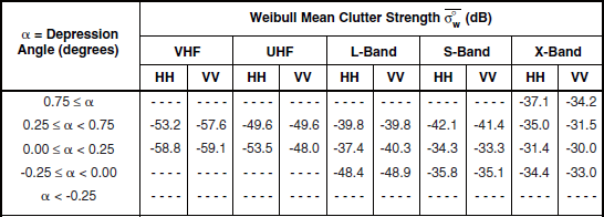

aTable 5.21 defines the population of terrain patches upon which these data are based.
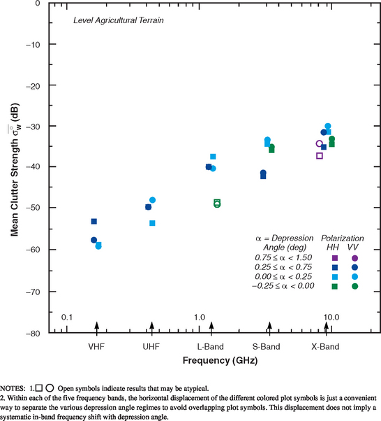
The weak, level farmland values of ![]() at VHF—in the −50 to −60 dB range—remain accurate, even though they are so weak. Almost all of the Phase One measured clutter histograms contain some samples at radar noise level. Mean clutter strength in the histogram is always computed two ways—first, as an upper bound, where the noise samples retain their noise power values, and second, as a lower bound, where the noise samples are given received power values equal to zero. The true value of mean clutter strength that would be measured by an infinitely sensitive radar, such that no noise samples would occur, must lie between these bounding limits. Only those measured clutter histograms are retained for which the differences between the upper bound and lower bound to mean clutter strength are < 1.5 dB. Usually these bounding estimates of mean clutter strength are within a small fraction of a dB. In any case, all values of mean clutter strength upon which Chapter 5 is based, even very weak ones, cannot be in error by more than 1.5 dB, and usually the error is much less. Coherent integration is utilized in processing the Phase One data to increase sensitivity to weak clutter returns (see Appendix 3.C).
at VHF—in the −50 to −60 dB range—remain accurate, even though they are so weak. Almost all of the Phase One measured clutter histograms contain some samples at radar noise level. Mean clutter strength in the histogram is always computed two ways—first, as an upper bound, where the noise samples retain their noise power values, and second, as a lower bound, where the noise samples are given received power values equal to zero. The true value of mean clutter strength that would be measured by an infinitely sensitive radar, such that no noise samples would occur, must lie between these bounding limits. Only those measured clutter histograms are retained for which the differences between the upper bound and lower bound to mean clutter strength are < 1.5 dB. Usually these bounding estimates of mean clutter strength are within a small fraction of a dB. In any case, all values of mean clutter strength upon which Chapter 5 is based, even very weak ones, cannot be in error by more than 1.5 dB, and usually the error is much less. Coherent integration is utilized in processing the Phase One data to increase sensitivity to weak clutter returns (see Appendix 3.C).
Now consider more closely what is happening in the level farmland ![]() data of Table 5.22 and Figure 5.22. First consider the dark blue, 0.25° to 0.75° results. On the level Corinne landscape, such relatively high depression angles occur only because of the effect of antenna mast height over very near-range clutter patches. Thus the dark blue, 0.25° to 0.75° results come from the five level clutter patches all in the 1- to 2-km range interval from the radar. Clutter returns from these near-range clutter patches are clearly discernible well above system noise level at all five Phase One frequencies. However, clutter patches at longer ranges rapidly become too weak for Phase One measurement at the lower frequencies due to multipath loss. Thus at VHF, of the seven patches in the 2- to 12-km range interval, only two provided clutter strong enough to be measured (given by the cyan, 0° to 0.25° results in Figure 5.22), and neither of the two longer range patches beyond 12 km were measurable above radar noise. At UHF, in addition to the five 1- to 2-km patches (dark blue, 0.25° to 0.75°), all seven patches between 2 and 12 km were measurable (cyan, 0° to 0.25°), but the two longer range patches continued to not provide measurable returns at UHF. At L-band, all 1- to 2-km patches (dark blue, 0° to 0.75°) and 2- to 12-km patches (cyan, 0° to 0.25°) remained measurable, and the single, 12- to 24-km patch at 100-ft higher elevation also became measurable (dark green, 0° to −0.25°). At S- and X-bands, all 14 patches provided valid measurements, including the longest range, 24- to 28-km patch; this last patch was also at 100-ft higher elevation and also contributes to the dark green, 0° to −0.25° results in these bands.
data of Table 5.22 and Figure 5.22. First consider the dark blue, 0.25° to 0.75° results. On the level Corinne landscape, such relatively high depression angles occur only because of the effect of antenna mast height over very near-range clutter patches. Thus the dark blue, 0.25° to 0.75° results come from the five level clutter patches all in the 1- to 2-km range interval from the radar. Clutter returns from these near-range clutter patches are clearly discernible well above system noise level at all five Phase One frequencies. However, clutter patches at longer ranges rapidly become too weak for Phase One measurement at the lower frequencies due to multipath loss. Thus at VHF, of the seven patches in the 2- to 12-km range interval, only two provided clutter strong enough to be measured (given by the cyan, 0° to 0.25° results in Figure 5.22), and neither of the two longer range patches beyond 12 km were measurable above radar noise. At UHF, in addition to the five 1- to 2-km patches (dark blue, 0.25° to 0.75°), all seven patches between 2 and 12 km were measurable (cyan, 0° to 0.25°), but the two longer range patches continued to not provide measurable returns at UHF. At L-band, all 1- to 2-km patches (dark blue, 0° to 0.75°) and 2- to 12-km patches (cyan, 0° to 0.25°) remained measurable, and the single, 12- to 24-km patch at 100-ft higher elevation also became measurable (dark green, 0° to −0.25°). At S- and X-bands, all 14 patches provided valid measurements, including the longest range, 24- to 28-km patch; this last patch was also at 100-ft higher elevation and also contributes to the dark green, 0° to −0.25° results in these bands.
Thus in Figure 5.22, with increasing frequency the clutter results come from patches enclosed within a gradually enlarging terrain region centered at the radar. This region is bounded by 4 km at VHF, 12 km at UHF, 24 km at L-band, and 28 km at S- and X-bands. Consider that, at VHF, the height to the peak of the first (1.5°) multipath lobe at 4 km is 105 m; obviously few clutter sources (e.g., farm buildings, grain storage silos, trees) reach this high, which explains the lack of discernible clutter beyond 4 km at VHF. In contrast, at X-band, the height to the peak of the first (0.03°) multipath lobe is only 6.3 m at 12 km. Thus at X-band, most clutter sources within 12 km are high enough to be fully illuminated. The strength of the illumination decreases with decreasing frequency from X-band.
The only common terrain region to all frequency bands in the results of Figure 5.22 is the close-range, 1 to 2 km region. Results from this close-range region are given by the dark blue, 0.25° to 0.75° plot symbols in Figure 5.22. Although the dark blue results generally show increasing clutter strength, VHF to X-band, they also show an S-band dip between L- and X-bands. The cyan, 0° to 0.25° results come from patches within the 2- to 12-km region, with fewer patches from within this region contributing at VHF than in the higher bands. The somewhat higher terrain beyond 12 km provides the dark green, 0° to −0.25° results. At L-band, these dark green results are shown as open plot symbols because they are based on single measurements. However, although relatively weak, these single L-band, dark green measurements may not be atypical, since at UHF and VHF the clutter returns from the terrain beyond 12 km drop to such low levels that they could not be measured with the Phase One equipment.
The purple, 0.75° to 1.5° results at X-band in Figure 5.22 are also shown as open plot symbols because they also come from single measurements. These results arose as follows. One of the patches in the 1- to 2-km region was at somewhat closer range than the others and had a depression angle close to 0.75°. In these particular (purple) X-band measurements of this patch which are at high range resolution, the precise positions of the range gates on the ground together with the precise X-band antenna height (slightly higher than the other bands) were such as to cause the depression angle to just exceed 0.75° (viz., 0.78°). For the corresponding low resolution X-band measurements of this patch, the range gate positions were at somewhat greater distances, and the depression angle was less than 0.75° (viz., 0.71°). Thus the low resolution X-band measurements from this patch are included in the dark blue results in Figure 5.22, as are all other measurements of the patch.
Similar migration of particular patch measurements across depression angle regime boundaries occasionally happens elsewhere in the results of Chapter 5. Specific discussion of individual sites such as is given here for Corinne is not possible in most other results of Chapter 5, which are generally based upon numerous sites in each terrain category. However, specific discussion of repeat sector results by individual site is given for many sites (including Corinne) in Section 3.4.
Shape Parameter aw. Table 5.23 presents the Weibull shape parameter aw and ratios of standard deviation-to-mean and mean-to-median for clutter amplitude distributions in level agricultural terrain by depression angle and radar spatial resolution. The statistical populations underlying the data of Table 5.23 are shown in Table 5.21. Since the level farmland results of Chapter 5 come from just one site (viz., Corinne), the populations shown in Table 5.21 are much lower than for most other terrain types. Table 5.23 shows that very large values of spread occur in spatial clutter amplitude distributions at low angles and high resolution in level agricultural terrain. For example, at near grazing incidence (i.e., 0° to 0.25° depression angle) and at high resolution (i.e., A = 103 m2), ratios of mean-to-median and standard deviation-to-mean of 36.4 and 13.4 dB, respectively, indicate a very highly skewed distribution.
TABLE 5.23
Shape Parameter aw and Ratios of Standard Deviation-to-Mean (SD/Mean) and Mean-to-Median for Level Agricultural Terrain, by Spatial Resolution A and Depression Angle*


aFootnoted values apply at A = 105 m2, not 106 m2.
*Table 5.21 defines the population of terrain patches and measurements upon which these data are based.
The main parametric trend of aw in Table 5.23 is with radar spatial resolution. In every case, aw is greater at 103 m2 resolution that at 106 m2 resolution. However, at the higher resolution of 103 m2, aw also strongly depends on depression angle. That is, in level agricultural terrain, although ![]() is largely invariant with depression angle, aw at high resolution decreases strongly from large values at grazing incidence (i.e., 0° to 0.25°) to much smaller values at higher angles.
is largely invariant with depression angle, aw at high resolution decreases strongly from large values at grazing incidence (i.e., 0° to 0.25°) to much smaller values at higher angles.
Each pair of aw numbers in Table 5.23 comes from a scatter plot of spread vs spatial resolution. The standard deviation-to-mean scatter plot for the 0° to 0.25° depression angle regime in Table 5.23 is shown in Figure 5.23. The data in Figure 5.23 show a very strong trend of decreasing spread with decreasing resolution (i.e., increasing A). There is a relatively small amount of measurement data underlying the scatter plot of Figure 5.23; see Table 5.16. In terms of plot symbols, Figure 5.23 is less populated than most similar scatter plots in Chapter 5, with results coming only from the first range interval at Corinne. The five individual frequency bands and the two pulse lengths per frequency band are easy to follow in these results. There is very tight correlation of these data to the regression line. These Corinne data strongly make the case, upon which all the results in Chapter 5 are based, that spread is predominantly affected by resolution and that direct effects of radar frequency on spread are small.
