
4.7 SUMMARY
Chapter 4 describes a number of approaches for modeling low-angle land clutter in surface-sited radar. As a physical phenomenon, the most salient attribute of low-angle clutter is variability. Two important ways in which this variability is evidenced are patchiness in spatial occurrence and extremely wide cell-to-cell statistical fluctuation in clutter strength (i.e., spikiness) within patches. A site-specific approach to clutter modeling is described based on the use of digitized terrain elevation data (DTED) at each site, which captures both of these basic attributes—patchiness, via deterministic computation of geometric terrain visibility from the radar site; and spikiness, via realizations from statistical distributions in which the spread depends on the depression angle to the backscattering terrain point as computed from the DTED.
An interim site-specific clutter model is provided as a table of Weibull coefficients in which the mean value of the distribution of clutter strengths varies with radar frequency, the shape parameter of the distribution varies with radar spatial resolution, and both mean strength and shape parameter vary with depression angle and terrain type. This site-specific approach to clutter modeling in surface radar is highly realistic. Besides capturing the fundamental patchiness and spikiness of low-angle clutter, this approach: (a) ensures that the modeled clutter in surface-sited radar dissipates with increasing range in the same way that clutter actually dissipates with increasing range at real sites, namely, via the deterministic visibility function, whereby the spatial patches of occurrence of clutter become fewer and farther apart with increasing range until, beyond some maximum range, no more clutter patches are visible; and (b) raises clutter modeling to the level of a quantitative science in that a given clutter patch at a given site, and, more specifically, the distribution of clutter strengths over that patch is a real and distinct physical entity that can be measured, parameterized (e.g., by terrain type and depression angle), and modeled, thus allowing quantitative comparison of the measured and modeled distributions and hence a direct means for clutter model validation.
Dominant sources of low-angle clutter appear to be of a point-like or spatially discrete nature, in that they occur in spatially isolated cells as opposed to being of a spatially extended nature. The basic site-specific approach to clutter modeling does not distinguish between whether clutter returns emanate from discrete or extended sources. A refinement to the basic site-specific clutter model is described involving a more computationally intensive approach that separates the modeling of dominant, locally strong clutter cells (called the discrete component) from weaker surrounding clutter cells (called the background component). Little correlation was found to exist between clutter cells that are locally stronger than their neighbors, and actual physical discrete objects on the terrain that could be identified as the sources of the strong clutter. Furthermore, it is not possible to determine in the measurement data whether a given, locally strong clutter return actually emanates from a definable, physical point object of specifiable RCS, or from a physically extended σ° clutter medium that by chance phasor reinforcement happens to produce a strong clutter return.
Therefore, the separate modeling of locally strong clutter cells under this approach needed to be carried out, not as a deterministic RCS overlay, but as a second statistical σ° process in which, with a specified probability of occurrence, a given cell might have a “discrete” component added vectorally to its “background” component. That is, under this approach an investigator is not provided with a single value of σ° for a given terrain type and illumination angle, but is provided with two values of σ°, one for “discrete” clutter and one for “background” clutter. The total clutter return is comprised of two components requiring two random draws, compared to modeling the total return as a single component obtained from one random draw.
In the separation of locally strong clutter cells from the weaker surrounding cells, the weaker clutter was found to be dependent at the resolution cell level on terrain slope and grazing angle, thus allowing the effect of landform on the weaker clutter to be provided at the cell level via computation of grazing angle using DTED rather than through macropatch classification of terrain relief; the locally strong (i.e., dominant) clutter, like the total clutter in the interim model, did not show correlation with grazing angle at the cell level. Another refinement to the basic site-specific clutter model obtainable with more intensive computation is the softening or blurring of shadow boundaries, as determined geometrically from DTED, whereby clutter is allowed to rapidly diminish into shadowed regions with increasing depth of shadow rather than abruptly terminating right at the shadow boundary.
These site-specific approaches to clutter modeling allow the limiting effects of clutter on radar system performance at any given site to be determined to a high degree of exactitude, thereby meeting much in the way of design- and analysis-related need for quantification and prediction of radar performance in ground clutter. In today’s highly evolved and rapidly expanding era of high performance computer capability, the fact that a site-specific approach to clutter modeling is computer-dependent, requiring extensive computation based on accurate DTED for the sites in question, is no longer very restrictive, whether concern is with individual sites or complexes of sites. The nature of ground clutter is that it can affect radar performance very differently from site to site, as a consequence of the extreme variations in surrounding terrain that can occur from one site to another, and a quantitative approach to the accurate assessment of the effects of clutter needs to reflect this specificity.
Nevertheless, the fact remains that the site-specific approach to modeling clutter provides answers one site at a time. For radar system design/analysis that requires more general information of the impact of ground clutter on system performance, the rigorous way under the site-specific approach is to first compute performance across a set of sites as specified by the particular design or analysis under consideration, and then to generalize (e.g., medianize) performance depending on how site-to-site performance varies across the set. Note that this approach to generality a posteriori averages the performance measures obtained from a number of realistic site-specific clutter computations; it does not attempt to a priori average the clutter first (a non-verifiable undertaking) followed by a one-time assessment of performance.
As a conceptual alternative to accepting the computational burden required in such a rigorous approach to generality, the idea of a clutter model that retains the important element of spatial patchiness but realizes it by means of a generic stochastic process in which patch extents, separations, and obliquities are statistically representative of general types of terrain rather than specific sites is intuitively attractive. This idea, involving implementation of generalized stochastic patchiness, although beyond the range of subject matter covered in this book, was explored at some length in coordinated studies involving the Lincoln Laboratory clutter data carried out by other investigative agencies ([3] is an early citation from extended research undertaken to develop this idea). However, the specificity of terrain feature at the scale at which terrain feature affects low-angle terrain visibility and clutter patchiness makes it difficult to capture such effects statistically. Unlike the ocean, the terrain at most sites of any significant relief is not very statistical in the sense of generally repeated patterns, but is dominated by a relatively few discrete singular macrofeatures (e.g., a mountain range, a ridge of hills, a river valley, a coastal shoreline). As a result, the parameters affecting the patchiness provided by a general stochastic model could not be related to simple quantifiable measures (e.g., surface relief; correlation distance) associated with generalized terrain types; but rather required that the parameters governing patchiness be acquired by an initialization or conditioning cycle of processing in DTED over a large-scale region encompassing the site of interest.
Such generalized approaches to stochastic patchiness were reasonably successful for terrain of relatively low or moderate relief; high-relief terrain is too specific for a stochastic approach to be appropriate. Since a stochastically patchy non-site-specific clutter model requires initialization using DTED from the terrain region of interest, the sought for advantages of such a model in providing non-site-specific stochastic realizations of patchiness are somewhat diminished compared with more straightforwardly obtained site-specific realizations of patchiness. For such reasons, the initially attractive and deceptively simple notion of a generic non-site-specific clutter model invested with realistic stochastic patchiness becomes more difficult to successfully implement in actual practice than might be presupposed, although a remaining advantage of the stochastically patchy approach is that it can lead to generic analytic formulations of such system performance measures as, for example, signal-to-clutter ratio vs range for the terrain type under consideration.
A spatially patchy clutter model, whether site-specific or non-site-specific, captures the important element of disconnectedness in spatial occurrence of low-angle terrain visibility that leads to a high degree of fidelity in the representation of ground clutter in surface radar. Such a high degree of fidelity is not always required, however, in the representation of ground clutter by radar system engineers. As a first indication of the effects of ground clutter, the radar system engineer may not be interested in the full-blown system effects of patchiness, but may require only a single value of constant σ° indicating how strong the clutter is at a given site for use in the radar range equation to estimate signal-to-clutter ratios against particular targets; and in addition may require only a single value of cut-off range to indicate the maximum extent in range to which the constant σ° applies and beyond which the radar is clutter-free.
From this point of view, the modeling of patchiness in low-angle terrain visibility may be regarded as a higher order (although important) effect in low-angle clutter phenomenology compared with modeling the strength of the clutter (assuming that the ground is visible), and for a beginning all that is required of this higher-order effect is a global estimate of the maximum extent of the patchy terrain visibility in range. Furthermore, this point of view disregards the fact that low-angle σ° occurs as a statistical phenomenon with wide cell-to-cell variations over a local region, but instead focuses on a single measure of strength such as the mean level; it also disregards the fact that σ° varies with depression angle since depression angle varies most significantly only within the first few kilometers of range from the radar, and usually diminishes to very near grazing incidence (e.g., 0.1° or 0.2°) over the much greater extents of clutter spatial occupancy that occur at much longer ranges.
To meet these kinds of less demanding requirements in a clutter model, Chapter 4 also provides a simple, non-patchy, non-site-specific clutter model that specifies mean clutter strength ![]() depending only on general terrain type (e.g., rural/low-relief, rural/high-relief, urban) and clutter cut-off range Rc depending only on effective radar height (e.g., low, intermediate, high). Since low-angle clutter is so variable both in strength and extent, these two parameters
depending only on general terrain type (e.g., rural/low-relief, rural/high-relief, urban) and clutter cut-off range Rc depending only on effective radar height (e.g., low, intermediate, high). Since low-angle clutter is so variable both in strength and extent, these two parameters ![]() and Rc are provided not only as baseline central values, but also as worst-case values indicative of severe or heavy clutter situations, and as best-case values indicative of benign or light clutter situations.
and Rc are provided not only as baseline central values, but also as worst-case values indicative of severe or heavy clutter situations, and as best-case values indicative of benign or light clutter situations.
A very large step in simplification occurs between the extremes of clutter models (viz., the full-blown site-specific statistical model vs the simple non-site-specific constant-σ° model) described in Chapter 4. Many of the difficulties that face efforts to bring realism to empirical clutter models at intermediate levels of fidelity between these two extremes are explored in ancillary discussions of the measured clutter data both in the body of Chapter 4 and its appendices. These ancillary discussions include considerations of (a) the inherent effects on terrain visibility and clutter strength of radar height and radar range; (b) the proper way to deal with unavoidable noise-level samples in clutter measurements and the important consequent effect on clutter statistics of rapidly decreasing radar sensitivity to clutter with increasing range; and (c) the wide range of variability involved in general clutter amplitude statistics and the attendant difficulty in specifying any particular σ° level for a constant-σ° clutter model.
Discussions are also provided concerning the relationship between terrain visibility and clutter occurrence and concerning discrete vs distributed clutter and the appropriate parameter by which to characterize low-angle clutter. All these discussions serve to more fully describe the complex, multifaceted nature of low-angle clutter from different perspectives and to bring home the value of the site-specific approach to clutter modeling in that it automatically and accurately incorporates all the complicating factors that are difficult for more general modeling approaches to capture. Although the main subject of Chapter 4 is the consideration of various approaches to modeling the spatial amplitude statistics of low-angle ground clutter, brief consideration is also given to aspects of the phenomenon associated with its temporal variability and its spectral and correlative properties.
Appendix 4.A CLUTTER STRENGTH VS RANGE
4.A.1 Introduction
An important characteristic of land clutter in a surface-sited radar as first perceived on the radar’s PPI display is that its occurrence dissipates rapidly with increasing range from the radar. Cannot this obvious general characteristic be simply modeled? The PPI display shows the spatial occupancy of the clutter, but otherwise (without introducing an intensity dimension to the basic plan-position display) does not directly show clutter strength within occupied regions. A simple, azimuthally-isotropic, non-spatially-patchy clutter model provides clutter everywhere and hence does not have variable clutter occurrence as an available parameter by which to properly diminish the clutter with increasing range. Clutter strength being the only available parameter of such a simple model, the question arises as to whether diminishing clutter strength with increasing range is a suitable way to provide the obvious general dissipation of clutter with increasing range as first perceived on a PPI display.
The correct way to answer this question is to look for such effects in measured clutter data. Thus Appendix 4.A shows mean clutter strength as a function of range at six selected sites. The basic A-scope or sector display format in which clutter strength variation is shown vs range is complementary with PPI clutter map presentations in advancing comprehension of the low-angle clutter phenomenon, so that besides addressing the basic question of clutter strength vs range, these results also provide additional insight into the general nature of low-angle clutter. Specifically, the sector display format shows the spikiness, clumpiness, and heterogeneity of clutter in which wide dynamic range in clutter strength is evident. This format shows from another perspective how low-angle clutter is dominated by discrete sources and provides intuitive understanding of why low-angle clutter often spatially decorrelates in one resolution cell. Furthermore, this format provides graphic evidence that low-angle clutter is essentially a line-of-sight phenomenon; where terrain is within line-of-sight, clutter spikes are observed occurring above the radar noise floor, and where terrain is geometrically masked, the return is usually at or near the noise floor. The data in Appendix 4.A show no significant general trends of decreasing strength with increasing range that could be incorporated as the basis of a simple non-patchy clutter model.
Table 4.A.1 lists the sites for which sector display results are shown in this appendix. The criterion for their selection was that ground clutter be discernible to relatively long-range. As a result, all six of these sites are of relatively high effective site height. For each site, a narrow azimuth sector was selected containing clutter to long-range, and a sector display was generated showing clutter strength vs range, range gate by range gate, from the beginning to the end of the sector. Figures 4.A.2–4.A.8 show these sector displays. Also shown in each of these figures is a Phase Zero PPI clutter map at close to (i.e., 3 dB from) full sensitivity in which the azimuth sector for which sector display results are presented is indicated.


FIGURE 4.A.2 Phase Zero sector display plot for Katahdin Hill showing σ°F4 vs range between 270° and 290° azimuth. Available dynamic range is indicated by solid lines bracketing the data. Mean (upper bound) and 99-percentile levels are shown for each range gate, averaged over 86 azimuth samples. Mean deviation is the difference between upper and lower mean bounds. A Phase Zero clutter map (clutter is black) is also shown, indicating the azimuth sector under consideration. The clutter map is 3 dB from full sensitivity; maximum range = 23.5 km; 5-km range rings; north is zenith.
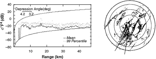
FIGURE 4.A.8 Phase Zero sector display plot for Blue Knob showing σ°F4 vs range between 190° and 210° azimuth. Mean (upper bound) and 99-percentile levels are shown for each range gate, averaged over 87 azimuth samples. Mean deviation is the difference between upper and lower mean bounds. A Phase Zero clutter map (clutter is black) is also shown indicating the azimuth sector under consideration. The clutter map is 3 dB from full sensitivity; maximum range = 47.1 km; 10-km range rings; north is zenith.
4.A.2 CLUTTER VISIBILITY VS RANGE
The six sectors in this appendix are selected at relatively high sites so as to contain significant amounts of clutter. Although selected in this manner to avoid the occurrence of macroshadow where the radar is at its noise floor over large spatial regions, nevertheless, and as typically occurs in ground clutter returns especially at longer ranges, a large amount of microshadowing occurs within the sectors. For each sector, the percent of cells at or within 3 dB of the noise floor is quantified as a function of range in Figure 4.A.1. This is done in two ways. First, the percentage of cells in clutter (i.e., the complement of percentage of cells at or near noise level) at each range gate position over the azimuthal extent of the sector is shown, range gate by range gate, across the 320 Phase Zero range gates in each sector. This quantity is denoted as percent circumference (or more precisely, percent of circumferential arc length spanning the azimuth extent of the sector) in clutter. The number of azimuth samples in each range gate for each of the six sectors is shown in Table 4.A.1. Second, the percentage of cells in clutter included within the sector out to and including the range under consideration is shown, also range gate by range gate across the 320 range gates in each sector. This quantity is denoted as percent of area in clutter (more precisely, it is the percentage of included cells in clutter—the percentage of included cells is not proportional to included area because cell area is range dependent). The quantity indicated as percent area in clutter is the cumulative sum of the quantity indicated as percent circumference in clutter from the first range gate out to the range gate under consideration.

FIGURE 4.A.1 Percent of included circumferential arc length and percent of included area in clutter for selected sectors at six sites. Phase Zero X-band data.
In Figure 4.A.1, all sectors show an initial rapid decrease, followed by a slower falloff, of percent of cells in clutter with increasing range. The details of this variation depend on the specific nature of the terrain and the effective radar height at each site. In all six cases, the percent of cells in clutter throughout the complete sector to its maximum range varies from about 10% to about 35%. That is, over such long ranges, the majority of cells occur at or near noise level, even within sectors selected to contain substantial amounts of clutter. The effects of these noise level cells on the mean clutter strength computed range gate by range gate in each sector are ascertained through computation of upper and lower bounds to mean clutter strength (see Appendices 2.B and 3.C) in selected range gates. The differences between these bounds are labelled as “mean deviation” for these selected range gates in Figures 4.A.2–4.A.8.

FIGURE 4.A.3 Phase Zero sector display plot for Picture Butte II showing σ°F4 vs range between 144° and 147° azimuth. Mean (upper bound) and 99-percentile levels are shown for each range gate, averaged over 14 azimuth samples. Mean deviation is the difference between upper and lower mean bounds. A Phase Zero clutter map (clutter is black) is also shown indicating the azimuth sector under consideration. The clutter map is 3 dB from full sensitivity; maximum range = 23.5 km; 5-km range rings; north is zenith.

FIGURE 4.A.4 Phase One sector display plot for Picture Butte II showing ![]() vs range between 147° and 150° azimuth. Mean clutter strength is shown for each range gate, averaged over 375 azimuth samples. A Phase Zero clutter map (clutter is black) is also shown indicating the azimuth sector under consideration. The clutter map is 3 dB from full sensitivity; maximum range = 47.1 km; 10-km range rings; north is zenith.
vs range between 147° and 150° azimuth. Mean clutter strength is shown for each range gate, averaged over 375 azimuth samples. A Phase Zero clutter map (clutter is black) is also shown indicating the azimuth sector under consideration. The clutter map is 3 dB from full sensitivity; maximum range = 47.1 km; 10-km range rings; north is zenith.

FIGURE 4.A.5 Phase Zero sector display plot for Cochrane showing σ°F4 vs range between 200° and 220° azimuth. Mean (upper bound) and 99-percentile levels are shown for each range gate, averaged over 87 azimuth samples. Mean deviation is the difference between upper and lower mean bounds. A Phase Zero clutter map (clutter is black) is also shown indicating the azimuth sector under consideration. The clutter map is 3 dB from full sensitivity; maximum range = 47.1 km; 10-km range rings; north is zenith.

FIGURE 4.A.6 Phase Zero sector display plot for Polonia showing σ°F4 vs range between 90° and 110° azimuth. Mean (upper bound) and 99-percentile levels are shown for each range gate, averaged over 86 azimuth samples. Mean deviation is the difference between upper and lower mean bounds. A Phase Zero clutter map (clutter is black) is also shown indicating the azimuth sector under consideration. The clutter map is 3 dB from full sensitivity; maximum range = 47.1 km; 10-km range rings; north is zenith.

FIGURE 4.A.7 Phase Zero sector display plot for Wachusett Mt. showing σ°F4 vs range between 45° and 90° azimuth. Mean (upper bound) and 99-percentile levels are shown for each range gate, averaged over 193 azimuth samples. Mean deviation is the difference between upper and lower mean bounds. A Phase Zero clutter map (clutter is black) is also shown indicating the azimuth sector under consideration. The clutter map is 3 dB from full sensitivity; maximum range = 47.1 km; 10-km range rings; north is zenith.
Over the set of 2,177 Phase Zero clutter patches lying between 2 and 12 km from the radar and upon which Chapter 2 is based, the percentage of cells at radar noise level is 47.1%. In the percent area results of Figure 4.A.1, the average percentage of included cells at radar noise level within these six sectors to 12-km range is indeed about 50% (i.e., on the order of the average clutter patch value), but increases to about 75% to the longest ranges shown. The increase in percentage of included cells at radar noise level in Figure 4.A.1 (i.e., the percent area curves) with increasing range is largely due to increasing geometrical shadowing of terrain with increasing range. Increasing geometrical shadowing with increasing range can theoretically result in gradually decreasing clutter strength with increasing range due to the spatial dilution of clutter cells with shadowed cells at noise level. In Figures 4.A.2–4.A.8, the mean strength in each range gate is accurate to the tolerances indicated by the mean deviation independent of sensitivity or number of noise samples in the range gate. No significant falloff of mean strength with increasing range occurs over the longer ranges in the sectors of Figures 4.A.2–4.A.8 because these sectors were selected to contain substantial discernible clutter, and as a result the occurrence of noise level cells in these sectors, although rising to relatively large values at long ranges, is not enough to significantly erode the accuracy of the mean strength computation or reduce it through spatial dilution.
Appendix 4.C discusses effects of shadowing and sensitivity on clutter strength in more detail. There, analysis is not restricted to narrow sectors of substantial clutter visibility, but instead large amounts of macroshadow are absorbed through 360° in azimuth. As a result, the percentage of cells at radar noise level rises to 99% at 47 km, and this constitutes enough spatial dilution to cause a significant reduction in mean clutter strength with increasing range (see Figure 4.C.16).
4.A.3 CLUTTER STRENGTH VS RANGE
Sector display plots showing clutter strength vs range at six sites are presented in Figures 4.A.2–4.A.8. These plots show clutter strength σ°F4 vs range, range gate by gate. The Phase Zero radar utilized 320 range gates (see Appendix 2.A). In each range gate, all of the clutter strength samples obtained from the beginning azimuth position of the sector to the ending azimuth position of the sector were binned in a histogram of clutter strengths. For each sector, the number of azimuth samples in the histogram is given in Table 4.A.1. Various statistical measures of this histogram were computed. In the sector display plots of Figures 4.A.2–4.A.8, the upper bound mean is shown as a solid line, and the 99-percentile level is shown as a dotted line. The noise floor or sensitivity limit is indicated as a monotonically increasing lower bound to the measurements which increases as the third power of range, and above it the saturation ceiling is indicated as a monotonically increasing upper bound to the measurements. These two limits define the available dynamic range of the clutter measurements.
Also indicated for a few range gate positions on most of these sector display plots are numbers labelled “mean deviation (dB).” The mean deviation indicates the difference between the upper and lower bounds to the mean, where in the upper bound computation, noise power values are assigned to samples at radar noise level; and in the lower bound computation, zero power values are assigned to these samples. Tight mean bounds indicate an accurate assessment of mean clutter strength to within the bounds indicated, irrespective of radar sensitivity or the number of corrupting radar noise samples involved in the calculation. The mean deviation also indicates to what extent significant clutter occurs in the range gate. In clutter patch selections to 12 km in range, the mean bounds are maintained within 1 dB of each other. The extent to which they drift apart beyond 1 dB in the sector display results of Figures 4.A.2–4.A.8 indicates to what extent macroshadowing begins to influence these results at longer ranges. In this appendix, narrow sectors containing relatively high spatial densities of clutter are selected to minimize macroshadowing. Appendix 4.C presents similar plots in which results are obtained by averaging over 360° to show the effects of macroshadowing and for which the upper and lower bounds to mean clutter strength are shown by individual range gate for all range gates.
For each sector display plot, depression angle was estimated at a few points in each sector from 1:50,000 scale or l:25,000 scale topographic maps; the results are indicated on the plots. At Katahdin Hill, the sector display of Figure 4.A.2 shows strongly decreasing mean strength as depression angle decreases from about 3° to about 1° in the first few kilometers in range. Similar effects are seen in the Cochrane and Wachusett Mountain results. However, in all of these sector display results, once the depression angle has dropped to < ∼1° in the first few kilometers, no further significant decrease of clutter strength with increasing range occurs. It is evident in these data that the controlling parameter on clutter strength is angle, not range, and that this effect of angle on clutter strength is of primary importance only within the first several kilometers of range from the radar. That is, once the depression angle falls off with increasing range into the near grazing incidence regime, then no further significant decreases of clutter strength occur with further extensive increases in range.
Picture Butte II. Picture Butte II is a prairie site for which terrain visibility occurs to very long distances, even though the site position is not on a local hill. The distant terrain remains visible due to long gradual terrain slopes such that terrain elevations gradually diminish over many kilometers to the southeast, as indicated in the terrain profile of Figure 4.A.9. Thus clutter occurs to long distances in the Picture Butte II sector unaccounted for by antenna mast height or local hill height, but simply because of geometric visibility down a long incline that overrides local earth curvature.

FIGURE 4.A.9 Picture Butte II terrain profile in southeast sector. Masked and unmasked terrain profiles are shown for 50-ft antenna.
Two Picture Butte II sector display results are provided. The first, shown in Figure 4.A.3, is a Phase Zero result to 23-km maximum range. In Figure 4.A.3, masked terrain in the Oldman River valley occurs from 9 to 13 km where the radar is at its noise floor; a cluster of buildings comprising the small village of Picture Butte occurs at 7-km range where mean clutter strength rises 20 dB over the surrounding cropland; and a small lake occurs at 6-km range where again the radar is at its noise level for a few gates. Next, Figure 4.A.4 shows an S-band Phase One sector display result for Picture Butte II to 44-km maximum range. In these S-band data, the polarization is horizontal and the range resolution is 150 m. The data were acquired in scan mode, scanning at 2°/s, at an effective PRF of 250 Hz. Thus in the 3° azimuth sector shown, each range gate receives 375 pulses. The mean strength shown is the result of binning 375 samples into an amplitude distribution for each gate and computing the mean of the distribution. The increased sensitivity of the Phase One radar compared to the Phase Zero radar is evident. The predominant character of the clutter on this agricultural landscape is similar in both Phase Zero and Phase One data. It is very spiky and discrete dominated, exhibiting wide dynamic range and occurring from terrain within line-of-sight. There is little suggestion of any significant general trend of σ°F4 with range to long ranges in these data.
4.A.4 SUMMARY
This appendix shows examples of mean clutter strength σ°F4 vs range for six high sites with clutter extending to long ranges. For each site, mean clutter strength is averaged over a number of azimuth samples within a fixed azimuth sector, range gate by range gate. In these results, a general trend of significantly decreasing clutter strength with increasing range is observed only over the first few kilometers, where depression angle significantly decreases with increasing range. At longer ranges where depression angle has very nearly reached zero degrees, mean clutter strength (although scintillating strongly from gate to gate) shows no general trend with range in the results.
Two conclusions concerning clutter modeling can be made from these results. First, since no strong general trend of decreasing σ° with increasing range occurs over long ranges in these data, the data provide no support to the idea of gradually dissipating clutter strength in a simple non-patchy clutter model by simply reducing σ° with increasing range. Second, even though low-angle clutter is dominated by discretes, the density function σ° normalized by cell area is the appropriate measure by which to characterize clutter strength. In contrast, clutter RCS per resolution cell does not isolate single discretes but generally increases approximately linearly with increasing range due to linearly increasing cell area (see related discussions in Section 4.5 and Appendix 4.D).
Appendix 4.B TERRAIN VISIBILITY AS A FUNCTION OF SITE HEIGHT AND ANTENNA MAST HEIGHT
4.B.1 Introduction
Ground-based radars are often situated on hills to improve their coverage. The relative height of the hill with respect to the surrounding terrain is an important parameter affecting the ground clutter received by the radar. Relative height directly affects the distance to which clutter occurs and indirectly, through illumination angle, affects the strength of the clutter received. These matters are discussed and illustrated with empirical data elsewhere in this book. In addition to the height of the hill itself, the antenna mast height of the radar also contributes to the overall effective height of the radar. In this book, a single height parameter is associated with the ground clutter data acquired at each clutter measurement site, namely, effective radar height, obtained by simply summing site height and mast height. Effective radar height is defined in Chapter 2, Section 2.2.3.
On first consideration, the summation of site height and mast height would appear to require little justification. However, raising mast height on a given site is not the same as moving to a higher site. In raising an antenna to higher positions at a given site, the surrounding terrain does not change, and simple geometrical considerations require that in such circumstances terrain visibility must monotonically increase with increasing mast height. Whereas, in moving to a higher site, the surrounding terrain does change, and, for example, terrain visibility at short ranges can decrease because the terrain slopes down the side of the hill upon which the radar is positioned can be increasingly shadowed for increasingly high hills. Except for very level terrain, increasing mast height through the ranges of practical heights typically used by ground-based radars only slowly increases visibility. The increases in long-range terrain visibility available from increasing site height are much greater than those available from increasing mast height.
For practical purposes, mast height is for the most part useful for raising the antenna into the clear above immediately surrounding vertical obstructions such as trees. However, in practice some very high radar antenna masts have been used purposefully to increase radar coverage of low-flying targets; and, in contrast, some very low radar sites have been purposefully selected to minimize terrain visibility and associated clutter effects in operations against high-altitude targets.
This appendix investigates effects of site height and mast height on terrain visibility. The investigation is based on geometric visibility of terrain as modeled by available digitized terrain elevation data (DTED) at 43 hilltop sites. The investigation provides generalized effects of site height and mast height on geometric line-of-sight visibility to terrain by averaging results across the 43 hilltop sites. To effect this process, first the sites are binned into four classes of site height, then terrain visibility results are averaged within class, and in this manner terrain visibility is generalized both by site height and mast height. As expected, the results show that increasing height on a given site monotonically increases visibility, although the rate of increase is usually small. The results also show that high sites see much more terrain at long ranges than low sites, and that this effect is much stronger than effects of mast height on visibility. However, the curves of visibility vs site height are not monotonically increasing.
This book associates the general spatial occurrence of the strongest elements of ground clutter with line-of-sight visibility to terrain. The study of terrain visibility of this appendix allows improved understanding of this association, in which low-angle ground clutter arises from discrete sources distributed over surfaces within line-of-sight visibility. In what follows, Section 4.B.2 describes the terrain elevation data employed in the study, and Section 4.B.3 provides the numerical results of the study.
4.B.2 TERRAIN ELEVATION DATA
This appendix uses DTED to characterize 43 hypothetical hilltop sites. These data are cartographic source data generated from 1:250,000 scale maps to provide terrain elevation in integer meters on an approximately 100 m grid. These DTED do not include tree heights or heights associated with any other land cover features. Thus, they are bare-earth DTED, and comprise a faceted terrain model as discussed in Section 1.2. The 43 sites were selected from a large contiguous geographic region approximately 1,000 km in extent, including plains and plateaus, uplands and lowlands. Hence, a considerable variety of terrain types is included within the set of sites, from relatively level to moderately hilly, although the study region does not include any mountainous terrain. Each of these sites was selected to be the highest hill within a radius of 10 km. These are hypothetical sites, in that no consideration was given to the practical accessibility of sites, or to whether or not there was any pre-existing utilization of the site for any purpose.
For each site, statistical computations on the DTED were performed. In particular, the relative height of each site was computed as site height above the best-fit plane over a 50 × 50 km site-centered area. This measure of relative site height is designated as site advantage. The resultant site advantages of all 43 hypothetical hilltop sites are plotted in increasing order of site advantage in Figure 4.B.1. Four regimes of site advantage and the number of sites in each from the 43-site set are shown in Table 4.B.1. These regimes are also demarcated in Figure 4.B.1. The next section shows terrain visibility results for each of the four regimes of site advantage shown in Table 4.B.1, averaged over the sites within each regime, and as a function of antenna mast height.

4.B.3 TERRAIN VISIBILITY RESULTS
This section presents terrain visibility results showing the effects of: (1) varying site height and (2) varying antenna mast height. Terrain visibility is shown as percent of circumference around site center in which the terrain is within line-of-sight visibility as a function of range. Percent of circumference visible as a function of range is computed from the DTED at each site through creation of a site-centered polar array of terrain elevation data of 80-km radius and grid spacing of 100 m by one deg. In the geometric determination of visibility of each point in this array, an earth of 4/3 the radius of the actual earth is used to account for standard atmospheric refraction. At each range position, the percent of circumference visible at each site is averaged together over all the sites within a given regime of site heights to provide the mean percent of circumference visible at that range for that site height regime. The computation of mean percent of circumference visible as a function of range for various site height regimes is performed for various antenna mast heights. This procedure generalizes terrain visibility as a function of relative site height and antenna mast height on the basis of the available 43-site set of DTED.
In these visibility computations, four antenna mast heights are used, as follows: (1) 5 m, (2) 15 m, (3) 30 m, and (4) 50 m. The 5-m mast height is rather low, for which visibility in many cases would be limited by land cover features. The 50-m mast height is a very high mast, impracticably so in most ground-based radar applications. Thus the 5-m and 50-m antenna mast heights approximate lower- and upper-bound limiting cases, whereas the 15-m and 30-m mast heights are of more practical interest. The four regimes of site advantage defined in Table 4.B.1 are of common occurrence.
Next, 16 curves are computed showing mean percent of circumference visible as a function of range for four site height regimes and four antenna mast heights. In each of these curves, visibility data is presented to a maximum range of 50 km. These curves are presented in two ways, as follows. First, in Figures 4.B.2–4.B.5, curves are shown for the four site height regimes in each figure, for a given mast height of 5, 15, 30, or 50 m, respectively. Then, in Figures 4.B.6–4.B.9, curves are shown for the four antenna mast heights in each figure, for a given site advantage regime of 10 to 35 m, 40 to 65 m, 70 to 95 m, or 100 to 200 m, respectively. Each curve includes an arrow indicating the horizon range on a smooth, spherical, 4/3 radius earth as seen from a height given by the sum of the antenna mast height and the median site advantage within the appropriate site advantage regime. If the spherical earth horizon range is greater than 50 km, it is not shown.
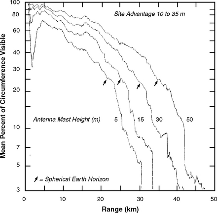
FIGURE 4.B.6 Mean terrain visibility vs range for four antenna mast heights, for sites with site advantage lying between 10 and 35 m. Based on bare-earth DTED for 43 hilltop sites.

FIGURE 4.B.7 Mean terrain visibility vs range for four antenna mast heights, for sites with site advantage lying between 40 and 65 m. Based on bare-earth DTED for 43 hilltop sites.

FIGURE 4.B.8 Mean terrain visibility vs range for four antenna mast heights, for sites with site advantage lying between 70 and 95 m. Based on bare-earth DTED for 43 hilltop sites.
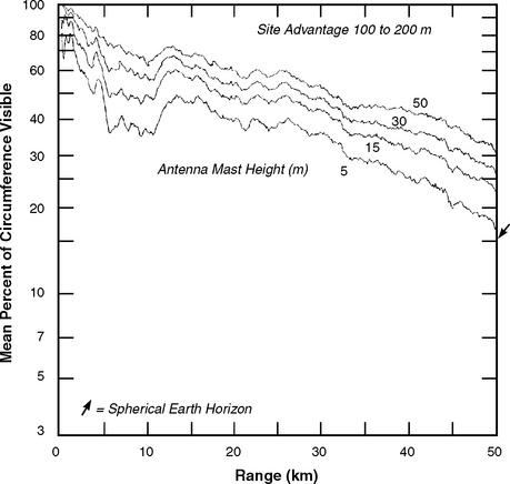
FIGURE 4.B.9 Mean terrain visibility vs range for four antenna mast heights, for sites with site advantage lying between 100 and 200 m. Based on bare-earth DTED for 43 hilltop sites.
Thus, Figures 4.B.2–4.B.9 directly show the effect on terrain visibility of either increasing site height for a given antenna mast height or increasing mast height for a given site height. Three important observations from these results are as follows:

FIGURE 4.B.2 Mean terrain visibility vs range for four regimes of site advantage, with a 5-m antenna mast height. Based on bare-earth DTED for 43 hilltop sites. The DTED are derived from cartographic source.

FIGURE 4.B.4 Mean terrain visibility vs range for four regimes of site advantage, with a 30-m antenna mast height. Based on bare-earth DTED for 43 hilltop sites.

FIGURE 4.B.5 Mean terrain visibility vs range for four regimes of site advantage, with a 50-m antenna mast height. Based on bare-earth DTED for 43 hilltop sites.
1. Higher masts incrementally increase terrain visibility at all ranges (see Figures 4.B.6–4.B.9). The influence of mast height on terrain visibility is stronger for low sites (Figure 4.B.6) than for moderate or high sites (Figures 4.B.7–4.B.9).
2. Higher sites strongly increase terrain visibility at long ranges (see Figures 4.B.2–4.B.5). This effect is generally much stronger than that of mast height at long ranges.
3. Increasing mast height on a given site is not the same as moving to a higher site. Increasing mast height gradually but monotonically increases terrain visibility at all ranges (Figures 4.B.6–4.B.9). Increasing site height results in slightly decreasing terrain visibility at short ranges, strongly increasing visibility at long ranges, and either slightly decreasing or slightly increasing visibility at intermediate ranges (Figures 4.B.2–4.B.5).
Observations 1 and 2, and the data supporting them, confirm intuitive expectation. Increasing mast height on a given site has to monotonically increase visibility, but this effect is relatively small for realistic mast heights. Furthermore, much more terrain in the distance must be visible from high sites than from low sites. This latter effect is stronger than the increased visibility obtainable through increasing mast height at a given site, high or low. This strong effect is largely due to the fact that high sites (e.g., 100 to 200 m) are much higher than high masts (e.g., 50 m), but the fact that high sites occur in high-relief terrain where the relief tends to dominate visibility to ranges far beyond a smooth spherical earth horizon also contributes.
Observation 3, however, is not so intuitive. The fact that, in moving to higher sites, terrain visibility actually decreases at short ranges (less than ∼10 km) is directly opposite to the effect caused by increasing mast height. Decreasing visibility with increasing site height at short-range is due to the “brow of the hill” effect whereby the terrain down the side of the hill upon which the radar is situated is masked to the radar. In contrast, for very low relief sites at short ranges, almost all of the terrain is visible. Since at long ranges (e.g., greater than 25 km for a 15-m mast height, see Figure 4.B.3) the expected effect of strongly increasing visibility with increasing site height comes into play, it is necessary that there be an intermediate range region in which site height has little effect and no clear-cut trend on visibility (e.g., between 10 and 20 km, high sites of 100 to 200 m site advantage and low sites of 10 to 35 m site advantage have about the same terrain visibility for 15-m mast heights, see Figure 4.B.3). Note that the “brow-of-the-hill” effect exists in the highest effective radar height regime in the 15-m mast clutter occurrence data of Figure 4.10, as well as in the highest site advantage regime in the corresponding 15-m mast terrain visibility data of Figure 4.B.3.
In Figures 4.B.2–4.B.5, the curves for the middle two regimes of site advantage (viz., 40 to 65 m, and 70 to 95 m) are not too different from each other and could be combined into one curve generally representative of most terrain. Further to this, it may be observed in Figures 4.B.2–4.B.5 that the upper envelope of all the visibility data is almost always given by the lowest (10- to 35-m site advantage) or highest (100- to 200-m site advantage) sites. Generally, lowest sites see most terrain at closer ranges, and highest sites see most terrain at long ranges. In these data, there is not a crossover range regime where sites of intermediate height see most terrain. On the other hand, there is a crossover range regime where sites of intermediate height (70- to 95-m site advantage) see least terrain. Otherwise, generally, highest sites see least terrain at close ranges, and lowest sites see least terrain at long ranges. Sites of 40- to 65-m site advantage never see most terrain or least terrain in these data.
Appendix 4.C EFFECTS OF TERRAIN SHADOWING AND FINITE SENSITIVITY
4.C.1 Introduction
This appendix investigates effects of terrain shadowing and radar sensitivity limitations on measurements of low-angle ground clutter strength. Shadowed terrain is terrain that is not directly illuminated or within geometrical line-of-sight to the radar. As range increases, the amount of terrain shadowing increases. Furthermore, as range increases, radar sensitivity decreases. For real radars with finite sensitivity limits, the increased terrain shadowing that occurs with increasing range is accompanied by increased numbers of samples at radar noise level in measured ground clutter distributions. These noise samples can introduce undesirable biases in clutter strength estimates. This appendix inquires into the effects of large numbers of noise samples on measured ground clutter distributions when large amounts of shadowing at long ranges occur. Section 4.C.2 shows the general qualitative effects to be expected of these influences on measured clutter distributions. In Section 4.C.3 clutter is reduced to long ranges within wide annular rings subsuming large amounts of shadow. In Section 4.C.4, clutter is reduced to long ranges within 360° range gates, similarly subsuming large amounts of shadow.
4.C.2 GENERAL EFFECTS ON MEASURED GROUND CLUTTER DISTRIBUTIONS
For a theoretically infinitely sensitive radar, increased terrain shadowing with increasing range can cause clutter strengths to decrease with increasing range because of the weak returns received from the shadowed cells illuminated only indirectly through diffraction. If strong clutter returns from visible regions are averaged together with weak clutter returns from shadowed regions, and if the shadowing is extensive, the resultant diminution of average clutter strength may be referred to as being caused by spatial dilution. That is, the strong clutter received from directly illuminated cells is diluted by spreading it out over many shadowed cells. This effect of spatial dilution of clutter strength is theoretically independent of sensitivity, although, practically, shadowed cells are often measured at radar noise level.
Real radars with narrow azimuth beams usually operate either within directly illuminated macroregions of visible terrain or free of strong clutter in macroregions of shadowed terrain; the radar receiver does not average together or spatially dilute strong clutter from visible regions with extensive amounts of weak clutter from shadowed terrain. Estimates of clutter strength within macroregions of visibility allow these estimates to remain on solid quantitative footing. The selection of clutter patches to lie in macroregions of clutter and not macroregions of shadow avoids their degradation by spatial dilution. Even within macroregions of visibility, many clutter return samples may occur on the noise floor of the radar. However, their numbers within patches are not so large as to prevent acceptable absolute measures of clutter strength from being obtained, either in terms of percentile levels in cumulative distributions, or in terms of mean strengths and higher moments (e.g., see Table 4.7, Figures 4.15, 4.16).
To achieve solid footing for estimates of clutter strength in the patch world in an absolute sense independent of radar sensitivity, all of the cells within the patch need to be included in the computation, including those for which the received clutter power measurement is at the noise floor of the radar. Appendix 4.A illustrates that within sectors that contain significant amounts of visible terrain, clutter strength does not diminish significantly with increasing range. This appendix moves beyond the patch world, such that very large numbers of noise samples are accepted into measured clutter distributions because of the inclusion of macroshadowing. Incorporation of large numbers of noise samples in the distributions requires careful interpretation of the results to avoid incorrectly assuming that observed relative biases caused by limited sensitivity are actual trends in absolute clutter strength.
Figure 4.C.1 shows sketches of clutter histograms including effects of noise and saturation. Here, as in Appendix 2.B, x is used to represent clutter strength σ°F4 in units of m2/m2, and y to represent 10 log10(x), i.e., y represents clutter strength in dB. Figure 4.C.1(a) shows an idealized sketch of a histogram of clutter strengths within some spatial region, as this histogram actually exists without reference as to how it might be measured. A perfect measurement radar with infinite dynamic range would measure this histogram, as shown in Figure 4.C.1(a), without introducing any spurious or contaminating effects. Note that Figure 4.C.1(a) shows definite limits both to the maximum clutter strength y*max (less than infinity) and the minimum clutter strength y*min (greater than zero) occurring in the histogram. Any actual histogram of measured clutter strengths is limited both in maximum and minimum in this way. On a dB scale for measuring clutter strength y, most theoretical distributions (e.g., Weibull, lognormal, K-) are not limited but stretch from minus infinity (i.e., zero power) to plus infinity. In what follows, the word “actual” is reserved to mean the distribution as it actually exists without reference to measurement considerations, as opposed to what is “measured” with a real radar limited in dynamic range.

All real radars are sensitivity limited. As a result, it is not unusual for some of the cells within a clutter region to be at the radar noise level. Thus many measured patch histograms are contaminated by noise at their weaker or lower levels. The noise samples do not all occur at a common clutter strength since the sensitivity limit is range dependent. Figure 4.15 shows examples of patch histograms with noise contamination where bins containing one or more noise samples are indicated with a double underline. In any measurement, it is known which samples are at radar noise level, so that they can be separated and dealt with as desired.
Besides overestimating the returns from weak cells at noise level, the radar may saturate on and thus underestimate the strength of some strong cells. Figure 4.C.1(b) shows a sketch representing the “measured” histogram of clutter strengths for the same clutter region for which the “actual” histogram of Figure 4.C.1(a) applies. The measurement is assumed to be performed by a real radar with limited dynamic range. In this measured histogram, the minimum measured strength ymin may be greater than y*min (i.e., ymin ≥ y*min) because of limiting from above at noise level, and the maximum measured clutter strength ymax may be less than y*max (i.e., ymax ≤ y*max) because of limiting from below at saturation level. The noise floor and saturation ceiling, in terms of absolute strength levels, are range dependent.
Figure 4.C.1(b) shows the strongest noise level sample reaching up into the histogram to a level denoted as ![]() In Appendix 2.B, Figure 2.B.2, this maximum noise level is designed as y’, and this designation is continued here for this important quantity. Similarly, the minimum saturation level is shown reaching down to a level denoted as
In Appendix 2.B, Figure 2.B.2, this maximum noise level is designed as y’, and this designation is continued here for this important quantity. Similarly, the minimum saturation level is shown reaching down to a level denoted as ![]()
To complete the nomenclature of various clutter strength levels, the minimum actual clutter strength measured above radar noise is denoted as ![]() , where
, where ![]() , and the maximum actual clutter strength measured below saturation is denoted as
, and the maximum actual clutter strength measured below saturation is denoted as ![]() where
where ![]() . In point of fact, saturation is usually much less a contaminating influence in clutter strength computation than noise, and, as indicated in the insert in Figure 4.C.1(b), often the highest bin in the histogram can contain both saturated and unsaturated samples, so that
. In point of fact, saturation is usually much less a contaminating influence in clutter strength computation than noise, and, as indicated in the insert in Figure 4.C.1(b), often the highest bin in the histogram can contain both saturated and unsaturated samples, so that ![]() . In what follows, the focus will be on noise contamination in considering effects of sensitivity limitations, requiring the use of y′ and
. In what follows, the focus will be on noise contamination in considering effects of sensitivity limitations, requiring the use of y′ and ![]() . Figure 4.C.1(c) shows a sketch of the “shadowless” histogram obtained as just the subset of measured samples from the histogram of Figure 4.C.1(b) containing discernible clutter above radar noise level.
. Figure 4.C.1(c) shows a sketch of the “shadowless” histogram obtained as just the subset of measured samples from the histogram of Figure 4.C.1(b) containing discernible clutter above radar noise level.
Figure 4.C.2 shows a sketch of the cumulative distribution function of the measured histogram of clutter strengths shown in Figure 4.C.1(b). This cumulative distribution function is obtained by integrating (or accumulating) across the histogram of Figure 4.C.1(b) left-to-right, but identical conclusions apply whether cumulative distributions are formed by integrating left-to-right or right-to-left across histograms. Many cumulative clutter distributions are shown in this book displayed on nonlinear Weibull or lognormal cumulative probability scales. All such cumulative distributions increase monotonically from zero at ymin to unity at ymax. In Figure 4.C.2 and elsewhere in this section, these limits of zero and unity are shown on the vertical cumulative probability scale, and for simplicity the cumulative distribution functions are shown to plot linearly (or piecewise linearly) against this otherwise arbitrary scale. Note that, as drawn in Figure 4.C.2, there is a break in slope in the measured cumulative distribution between the noise-contaminated region and the uncontaminated region. This is seen in many measured distributions. Since it is known in any measurement what the maximum measured noise clutter power level y′ is, the investigator may choose to only consider the uncontaminated upper region of the distribution at percentile levels greater than P′.

Suppose a particular clutter region is selected and repeatedly measured in steps of increasing sensitivity. The resultant clutter strength histograms would be as shown in Figure 4.C.3. As the sensitivity increases, the region of noise contamination is pushed to lower levels further to the left. The resultant cumulative distribution functions are shown in Figure 4.C.4 from which an important observation may be made. As the sensitivity increases, the measured distribution in Figure 4.C.4 matches the actual (unlimited sensitivity) distribution to lower and lower y levels. At any sensitivity, the cumulative distribution matches the actual distribution for (y, P) values greater than the (y′, P′) values at that sensitivity. This is one important reason why noise-level cells must be retained in measured clutter distributions. By doing so, absolute or sensitivity-independent percentile measures of clutter strength are obtained for y > y’. As shall be seen, distributions formed of only those samples above radar noise level within a region, or what are referred to here as shadowless distributions, do not have this attribute.


FIGURE 4.C.4 Behavior of measured cumulative distributions of clutter strength with varying radar sensitivity.
In working within a patch world of clutter amplitude statistics, an analyst keeps on solid footing by working with the complete distribution for any patch including samples at radar noise level. As discussed, doing so keeps percentile results sensitivity independent. That is, any percentile levels P so provided are absolute measures as long as P > P′. If P < P′, the corresponding clutter strength y < y′ is an upper bound to true or absolute clutter strength. It is the continuous sequence of increasing values of P with increasing y that forms the cumulative distribution function. These functions are valid absolute measures of clutter strength only over the uncontaminated region P > P′.
With respect to the moments (e.g., mean, standard deviation, etc.) of measured clutter patch amplitude distributions, which depend upon y < y′ as well as y > y’, the analyst keeps on solid footing by computing upper- and lower-bound estimates for each moment. The upper bound is computed by assigning y = ynoise to noise cells, where ynoise is range dependent. The lower bound is computed by assigning x = 0 power to all noise cells. For clutter patches in visible regions of terrain, these bounds are usually within a fraction of a dB of each other, even for large amounts of microshadowing (see Table 4.7). The reason the noise values have such little influence on moments of clutter amplitude statistics from patches is that the strong clutter cells dominate the computations. This would be more intuitively obvious if a linear abscissa x were employed, rather than a logarithmic abscissa y.
Close upper and lower bounds to amplitude moments do not always occur in investigations of clutter amplitude statistics. These bounds are close to each other in the patch world because patches are purposefully selected to contain substantial visible clutter. If these bounds drift apart from each other for a patch, it is an indication that the patch was poorly selected. However, when the patch world is departed from and macroshadowing is allowed to contaminate clutter amplitude distributions and measures of clutter strength, these bounds can be widely separated.
To provide some insight into these macroshadowing matters, consider the shadowless histograms of clutter strength sketched in Figure 4.C.5, as measured from a given clutter region by radars of increasing sensitivity. Shadowless distributions are formed of only those samples within a region above the radar noise level. When examining a large macroscopic region of spatial extent containing a high percentage of cells at radar noise level, an analyst may feel motivated to consider only the subset of shadowless cells in which actual ground clutter is discerned above radar noise level.

FIGURE 4.C.5 Behavior of measured shadowless histograms of clutter strength with varying sensitivity.
As shown in Figure 4.C.1(c), shadowless histograms contain only y values greater than ysigmin, and the typical secondary lobe due to noise contamination is not evident in them. Note that the number of samples in a shadowless histogram is sensitivity dependent, as shown in Figure 4.C.5. The more sensitive the measurement radar, the more cells in a given clutter patch that will be measured above the noise level. Thus, in Figure 4.C.5, the left side of the histogram extends further to the left and includes more samples with increasing sensitivity. Since the computation of moments (e.g., mean) of these shadowless distributions obviously depends on the number of clutter samples Nc above the noise level
moment computations of shadowless distributions are not fixed in any absolute sense, but vary with sensitivity. On the other hand, when the noise cells are included in the distributions as in Figure 4.C.1(b), there always exists a fixed total number of cells within the patch which are used in all upper and lower bound moment computations; thus, such computations are fixed as absolute measures independent of sensitivity.
Figure 4.C.6 shows how the cumulative shadowless distribution function for a given region varies as a function of sensitivity. The distributions sketched in Figure 4.C.6 are formed by integrating left-to-right across the shadowless histograms of Figure 4.C.5. Each distribution in Figure 4.C.6 begins to rise from P = 0 at the minimum discernible clutter strength level ysigmin applicable for a particular sensitivity. As a result, the shape or slope of the shadowless cumulative clutter distribution varies with radar sensitivity over the complete extent of the distribution. The shadowless distributions of Figure 4.C.6 may be compared with the distributions of Figure 4.C.4 which include noise samples and are not sensitivity dependent for (y, P) greater than (y′, P′). The sensitivity dependence of the shadowless distributions in Figure 4.C.6 is clearly undesirable.

FIGURE 4.C.6 Sensitivity dependence of shadowless distribution of clutter strengths for a given clutter patch.
Until now, this section has been considering how noise and sensitivity affect measures of clutter strength within a given clutter region. It has been shown that, for a given region of spatial extent with fixed boundaries, the resultant distributions of clutter strength within those boundaries are independent of sensitivity for y > y′ as long as they include the noise level cells. The question now raised is, what happens when those boundaries are allowed to vary? Imagine a hypothetical circular spatial region of strong clutter in which all cells are above radar noise level, as shown by region 1 in Figure 4.C.7. The cumulative clutter distribution for region 1 would be as shown (idealized) by the zero percent shadowing curve in Figure 4.C.8. Now let the boundary of the circular region expand to position 2 in Figure 4.C.4., in which all the cells in the additional annular region are at radar noise level. The cumulative clutter amplitude distribution for this larger region containing a low degree of shadowing is as indicated by the low percent shadowing curve in Figure 4.C.8. Similarly, if the circular boundary of the clutter region continues to expand to regions 3 and 4 as shown in Figure 4.C.7, the cumulative clutter distributions become noise contaminated to higher and higher percentile levels as shown in Figure 4.C.8.


As more and more shadowing is included within a region with a center core of discernible clutter, the uncontaminated part of the distribution of (y, P) greater than (y′, P′) changes shape or slope depending on the amount of shadowing included. Thus the distribution, even in its region of validity, is not absolute and independent of the choice of boundary. An important point emerges here. Measures and distributions of clutter strength within a clutter patch theoretically depend upon the selection of the patch boundaries. Only after the boundaries are set does the distribution within those boundaries, which includes the noise cells, become an absolutely specifiable quantity independent of sensitivity for y > y’. The theoretical dependence of clutter patch spatial amplitude distributions on selection of patch boundaries reflects the basic heterogeneity of terrain.
In actual practice, most clutter patch amplitude distributions are not too sensitive to boundary specification because patch boundaries are selected to encompass relatively uniform terrain regions such that small changes in boundaries usually do not cause abrupt changes in relative clutter and shadow densities within patches. Thus a patch world keeps an analyst on solid quantitative footing in this matter also, in that the specification of boundaries for most patches is not a major factor influencing shapes and strengths of resultant distributions. This is not the case in the following sections of this appendix, in which patch analysis is bypassed to allow consideration of clutter distributions containing increasingly large amounts of macroshadow with increasing range.
This section concludes by comparing the idealized clutter distributions of Figure 4.C.6 with those of Figure 4.C.8. In Figure 4.C.6, increasing sensitivity strongly affects the shape of the shadowless distribution for a fixed clutter region by moving the starting strength ![]() of the distribution increasingly to the left or to lower values. In Figure 4.C.8, increasing the relative amount of shadowing within a region while maintaining a non-changing shadowless core distribution of discernible clutter within the region strongly affects the shape of the resultant clutter distribution that includes radar noise cells. In this latter case, increasing shadowing affects the shape by moving the starting percentile level P′ of the uncontaminated range of the distribution y > y′ increasingly up the vertical scale to higher values. In the next section, it will be seen how the incorporation of increasing macroshadowing in measured cumulative clutter distributions with increasing range results in both of these strong effects associated with variations in sensitivity and shadowing undesirably influencing the shapes and strengths of the measured distributions.
of the distribution increasingly to the left or to lower values. In Figure 4.C.8, increasing the relative amount of shadowing within a region while maintaining a non-changing shadowless core distribution of discernible clutter within the region strongly affects the shape of the resultant clutter distribution that includes radar noise cells. In this latter case, increasing shadowing affects the shape by moving the starting percentile level P′ of the uncontaminated range of the distribution y > y′ increasingly up the vertical scale to higher values. In the next section, it will be seen how the incorporation of increasing macroshadowing in measured cumulative clutter distributions with increasing range results in both of these strong effects associated with variations in sensitivity and shadowing undesirably influencing the shapes and strengths of the measured distributions.
4.C.3 LONG-RANGE CLUTTER WITHIN WIDE ANNULAR REGIONS
The world of clutter patches, upon which much of the analysis of this book is based, avoids undesirable consequences of shadowing in estimates of low-angle ground clutter strength, even though some degree of shadowing is unavoidable even within patches (see Table 4.7). Although shadowing of clutter increases and radar sensitivity to clutter decreases with increasing radar range, the measures of clutter strength within patches remain absolute measures accurate at long ranges as well as short ranges. Such patch measures of clutter strength show no significant general trend with increasing range over the long ranges beyond that at which the onset of the grazing incidence depression angle regime occurs. This is shown in the sector display results of Appendix 4.A, in which the long-range narrow-azimuth sectors employed may be thought of as long narrow patches over largely visible terrain containing significant amounts of clutter. The work of patch selection eliminates macroshadow in estimates of clutter strength. If macroshadow is not eliminated, its effects intrude in analyses of clutter strength. This section and the next show how clutter strength varies with range, including the effects of macroshadow, either as the macroshadow occurs in wide annular rings in this section, or as the macroshadow occurs within individual range gates in the next section.
Ground clutter is now analyzed in large annular regions, using Phase Zero measurements at 47-km maximum range setting (see Appendix 2.A, Table 2.A.3). At this range setting, the radar RF pulse length is 1 μs, and the resultant range resolution is 150 m. Ten sites were selected, as listed in Table 4.C.1, of varying land cover, landform, and effective site height, but all with substantial amounts of measured clutter to long range. Measured PPI clutter plots to 47-km maximum range are shown for each site in Figure 4.C.9. Four annular regions were specified with range extents as follows: (1) 5 to 15 km, (2) 15 to 25 km, (3) 25 to 35 km, and (4) 35 to 45 km. For each of these four annular regions, all of the individual spatial samples of clutter strength from all 10 sites were aggregatively combined to form four ensemble histograms of clutter strength, each applying to a general annular region. Standard procedures for characterizing clutter amplitude statistics over spatial regions (see Appendix 2.B) were then applied to each of these four histograms.


FIGURE 4.C.9 Ground clutter maps at 10 sites, selected for investigating clutter strength dependencies on range. Phase Zero X-band data. In each map, maximum range = 47 km, north is zenith, range resolution = 150 m, clutter is black, clutter threshold is 3 dB from full sensitivity. Figure continued on next page.
Ground clutter maps at 10 sites, selected for investigating clutter strength dependencies on range. Phase Zero X-band data. In each map, maximum range = 47 km, north is zenith, range resolution = 150 m, clutter is black, clutter threshold is 3 dB from full sensitivity. Results above conclude this figure.
Figure 4.C.10 shows the resultant four cumulative amplitude distributions, each one containing all measured samples over 10 sites within the indicated range interval or annular region, including all samples at radar noise level. There is an obvious trend in the relative shapes and positions of these distributions with increasing range. Table 4.C.2 shows some statistical attributes of these four distributions which help provide understanding of how clutter strength varies across these distributions. First, the 99-percentile level shows a clear trend of decreasing strength with increasing range. This trend reflects the fact that the relative positioning of these distributions is ordered by range, with the long-range distribution left-most (i.e., weakest), and the short-range distribution right-most (i.e., strongest) in Figure 4.C.10. This trend, however, is primarily just a direct consequence of the relative number of samples at radar noise level in each distribution. As is shown in Table 4.C.2, the percent of samples at radar noise level increases strongly with increasing range, from 54% at short-range to 97% at long-range. Clearly, as a radar looks out to longer and longer ranges, it will see less and less clutter above its sensitivity limit, and this will always drive any given percentile level of clutter strength down with increasing range, until, in the limit at long enough range, all percentile levels lie on the noise floor.
TABLE 4.C.2
Clutter Strengths by Annular Regiona Including Noise-Level Samples

aAveraged over ten sites, see Table 4.C.1.
bLower percentiles are noise contaminated.
cComputed in units of m2 /m2 and subsequently converted to dB.
dNoise samples assigned noise power values.
eNoise samples assigned zero power values.
fRange sample interval = 148.41 m; azimuth sample interval = 0.234°.

FIGURE 4.C.10 Cumulative distributions of clutter amplitude statistics, conglomeratively combined from 10 sites into four annular regions. These four distributions include all spatial samples including those at radar noise level. The distributions are shown only as they emerge to the right of their noise-contaminated regions for σ°F4 levels greater than the maximum σ°F4 level in which noise occurs in each distribution. Phase Zero X-band data, 150-m range resolution. Compare with Figure 4.C.8.
The ordered positions with range of the distributions in Figure 4.C.10 are explained by the sketch of Figure 4.C.8. The latter indicates how distributions vary when a central core of clutter is surrounded by more and more shadow. This is similar to the situation with the four annulae of measured data, where, as range increases, the samples of discernible clutter are immersed in more and more macroshadow. Thus, the relative positions of the distributions in Figure 4.C.10 are primarily controlled by macroshadowing. Recall that these distributions, as shown in Figure 4.C.10 only above their regions of noise contamination y > y′, are sensitivity independent and reflect absolute levels, as do those in Figure 4.C.8.
Next, consider the mean strengths of the clutter distributions in Figure 4.C.10. Upper and lower bounds to the mean strengths of these distributions are included in Table 4.C.2. Consideration of upper and lower bounds keeps analysis on solid footing here in the face of macroshadowing, as it does within patches in the face of microshadowing. In either case, an infinitely sensitive radar that would measure discernible clutter return in every resolution cell (i.e., no noise samples) would find a mean clutter strength between these bounds. Overall, the mean bounds shown in Table 4.C.2 indicate decreasing mean clutter strength with increasing range. If an infinitely sensitive radar looks to longer and longer ranges, the mean clutter strength must eventually strongly decrease as more and more cells become lit only by diffraction.
The percent of samples at radar noise level in the outer two annulae is 94% in the 25- to 35-km annulus and 97% in the 35- to 45-km annulus. Since the total number of samples combined from 10 sites in each annular region is large (i.e., approximately 106, see Table 4.C.2), even small percentages of discernible clutter samples (i.e., 6.2% in the 25- to 35-km annulus; 2.6% in the 35- to 45-km annulus) still result in sizeable sample populations of clutter (66,138 clutter samples in the 25- to 35-km annulus; 27,169 clutter samples in the 35- to 45-km annulus) from which general conclusions may be drawn regarding clutter strength vs range.
Figure 4.C.11 shows the four cumulative shadowless clutter amplitude distributions that result from collecting just the samples in these annulae in which discernible clutter occurs above the noise floor. Each distribution in Figure 4.C.11 contains all samples of discernible clutter from 10 sites within the indicated range interval. No samples at radar noise level are included in these shadowless distributions. Here, as in Figure 4.C.10, an obvious trend is seen in the relative shapes and positions of these shadowless distributions, although each is quite different from its counterpart in Figure 4.C.10.

FIGURE 4.C.11 Cumulative distributions of shadowless clutter amplitude statistics, conglomeratively combined from 10 sites into four annular regions. These distributions include only those spatial samples in which discernible clutter above the radar noise floor was measured. Phase Zero X-band data, 150-m range resolution. Compare with Figure 4.C.6.
Table 4.C.3 shows some statistical attributes of these shadowless distributions. There is a clear indication of increasing clutter strength with increasing range in these shadowless clutter statistics. The true trend of decreasing clutter strength with increasing range as would be measured by an infinitely sensitive radar is masked in these shadowless data by the effects of decreasing sensitivity with increasing range. This is seen by comparing the actual empirical shadowless distributions of Figure 4.C.11 with the idealized shadowless distributions sketched in Figure 4.C.6. The latter indicate how shadowless distributions vary with decreasing sensitivity for a given clutter region. This idealized variation as sketched in Figure 4.C.6 explains the dominant trend observed with range in the distributions of Figure 4.C.11.
TABLE 4.C.3
Shadowless Clutter Strengths by Annular Regiona

aAveraged over ten sites, see Table 4.C.1.
bThese are not true σ°F4 statistics but are conditional on clutter strength being above noise level. For example, multiplying mean σ°F4 given here by cell area does not yield true mean clutter cross section or allow the computation of the true mean clutter power.
cComputed in units of m2/m2 and subsequently converted to dB.
We wish to determine how ground clutter strength varies with range in an absolute sense not dependent on radar sensitivity. The data of Figure 4.C.10, although absolute measures, are biased by spatial dilution; these data are dominated by the fact that as a radar looks to longer ranges, it sees increasingly less ground clutter and is at its noise level over increasingly large spatial regions. If, as in Figure 4.C.11, we attempt to resolve this problem by considering only discernible clutter samples above radar noise level, these shadowless data are also biased (i.e., they are relative, not absolute, measures), dominated by the fact that radar sensitivity decreases with range so that at far ranges the radar only measures very strong clutter. Working with clutter strengths within visible terrain patches and employing a model that keeps separate the ideas of where the clutter is and how strong it is avoids such problems.
In what follows, the analysis of ground clutter within large annular regions is continued in order to find an unbiased answer in these results on how clutter strength varies with range, such that the strong biasing effects caused by increasing shadowing and decreasing sensitivity with increasing range are normalized out. To do this, shadowless statistics are employed but the same radar sensitivity is artificially enforced in all annulae as exists in the farthest range annulus. That is, the radar sensitivity is decreased in the first three annulae to equal that in the fourth annulus. In Figure 4.C.10, which shows the distributions only above the maximum noise-contaminated bin y > y′ [see Figure 4.C.1(b)], the maximum noise-contaminated bin in the 35- to 45-km annulus is σ°F4 = −27 dB. Thus, for each annular regime, the distributions are formed of all clutter samples of measured strength σ°F4 ≥ −24 dB, thereby providing a buffer of 3 dB to be well clear of the noise in the 35- to 45-km regime.
The resultant distributions are shown in Figure 4.C.12. They are very nearly identical. They indicate that strong clutter, as it occurs for σ°F4 ≥ −24 dB, exists independently of range from the radar. This annular region result is necessarily restricted to apply only to strong clutter in order that it avoid biases introduced by effects of varying sensitivity or degree of shadowing with range. Table 4.C.4 provides some additional quantitative measures of the distributions shown in Figure 4.C.12. These measures reinforce the obvious range-independence of the data in Figure 4.C.12. Care must be taken in the use of these conditional data in Figure 4.C.12 or Table 4.C.4, since they portray only conditional σ°F4 statistics that occur equal to or stronger than −24 dB. In this respect, note that the conditional mean clutter strength values in Table 4.C.4 are much higher than the true unconditional means as indicated by the mean bounds in Table 4.C.2.
TABLE 4.C.4
Statistical Attributes of the Distributions of Clutter Strength of σ°F4 ≥ −24 dB, by Annular Regiona

aAveraged over ten sites, see Table 4.C.1.
bComputed in units of m2/m2 and subsequently converted to dB; these are not general spatial amplitude statistics but are conditional on σ°F4 ≥ −24 dB; multiplying mean of σ°F4 as given here by ground area does not yield true mean clutter cross section.
cSaturated.

FIGURE 4.C.12 Cumulative distributions of clutter amplitude statistics with strength σ°F4 ≥ −24 dB, conglomeratively combined from 10 sites into four annular regions. These distributions include only those spatial samples in which σ°F4 ≥ −24 dB was measured. Phase Zero X-band data, 150-m range resolution.
Another way of showing the σ°F4 ≥ −24 dB data of Figure 4.C.12 is in the normalized histograms shown in Figure 4.C.13. These histograms are normalized to show the relative number of samples at a given σ°F4 level greater than −24 dB compared to the number of samples at −24 dB. This normalization is in contrast to that of the cumulative distributions in Figure 4.C.12, which is with respect to the total number of samples of σ°F4 ≥ −24 dB. The data in both Figures 4.C.12 and 4.C.13 are strongly indicative of range-independence of clutter samples for which σ°F4 ≥ −24 dB. Many of these samples are doubtlessly caused by the existence of strong discrete backscattering sources on the landscape. There is no reason to expect that the distribution of such strong cells on the landscape would show any general preference with respect to range from the radar, and this is borne out by the data in Figures 4.C.12 and 4.C.13.

FIGURE 4.C.13 Normalized histograms of clutter amplitude statistics with strength σ°F4 ≥ −24 dB, conglomeratively combined from ten sites into four annular regions. These histograms contain only those spatial samples in which σ°F4 ≥ −24 dB was measured. Phase Zero X-band data, 150-m range resolution.
4.c.4 LONG-RANGE CLUTTER WITHIN 360° RANGE GATES
The previous section presented ground clutter data from 10 sites averaged azimuthally within four broad annular range rings to 45-km maximum range. In the analysis of these data, shadowing and sensitivity were major factors. This section expands these previous insights into range dependencies of measured clutter data by considering the same 10-site set of clutter data in the limiting case as an annular ring shrinks in width to a single range gate. Average clutter strength vs range is shown, range gate by range gate, to 47-km maximum range. This approach provides continuous range dependencies in the results. The constant radar noise level within each range gate allows a more straightforward determination of the effects of sensitivity on mean clutter levels. These results, like those of the previous section, continue to entail 360° azimuth averaging through macroshadow. The resulting spatial dilution of clutter strengths causes trends of decreasing clutter strength with increasing range in the results. These results apply to the hypothetical situation of a radar with an azimuthally omnidirectional antenna pattern in which mean clutter power levels received would, indeed, include effects of macroshadowing through 360°.
First, some analytical relationships are developed applicable to this range gate by range gate investigation. Assume that, in a given range gate from the radar, all azimuth samples from one complete azimuth scan of the radar are binned in a histogram and averaged. Let the total number of azimuth samples from one complete 360° azimuth scan be N. For the Phase Zero radar, N = 1,536 (see Appendix 2.A). The notation here follows that first developed in Appendix 2.B, where x represents clutter strength σ°F4 in units of m2/m2, and y = 10 log10 (x). Thus clutter strength from each of the N azimuth samples is represented as xi, i = 1 to N. The overall mean of these N samples, denoted ![]() , is given simply by
, is given simply by
Of these N samples, some will be true measurements of clutter strength above the sensitivity of the radar at that range, and some will be at the noise floor of the radar due to shadowing. Suppose there are Nc true measurements of clutter, and Nn measurements at noise level. Then, N = Nc + Nn. The ratio Nc/N is the fraction of the circumference in clutter at the range gate under consideration. That is, the quantity (Nc/N × 100) is what is referred to as percent circumference in clutter elsewhere in this book (see Section 4.3.2, Figures 4.8 and 4.10). If xi is a true clutter measurement, let it be represented by ![]() , and if xi is a noise measurement, let it be represented by
, and if xi is a noise measurement, let it be represented by ![]() . With this, the mean of just the set of samples constituting true clutter measurements, which is denoted here as the shadowless mean, is given by
. With this, the mean of just the set of samples constituting true clutter measurements, which is denoted here as the shadowless mean, is given by ![]() , where
, where
Since at a given range, all Nn samples of noise are of equal clutter strength, the notation simplifies, as ![]() . With this terminology, Eq. (4.C.1) may be expressed as:
. With this terminology, Eq. (4.C.1) may be expressed as:
Now consider the meaning of the various terms and factors in Eq. (4.C.3). The shadowless mean ![]() is the mean of the clutter samples only, without any shadowed cells at radar noise level. It is obviously dependent on the sensitivity of the radar and hence range, and as a result is by itself not an absolute measure of clutter strength. When
is the mean of the clutter samples only, without any shadowed cells at radar noise level. It is obviously dependent on the sensitivity of the radar and hence range, and as a result is by itself not an absolute measure of clutter strength. When ![]() is multiplied by the fraction of circumference in clutter, however, the result is an absolute lower bound to the overall mean clutter strength in the range gate under consideration. This may be seen in Eq. (4.C.3), where there are Nn samples at the noise floor xn contributing to the overall mean
is multiplied by the fraction of circumference in clutter, however, the result is an absolute lower bound to the overall mean clutter strength in the range gate under consideration. This may be seen in Eq. (4.C.3), where there are Nn samples at the noise floor xn contributing to the overall mean ![]() . These Nn noise samples of strength xn are not true measures of clutter strength, but represent upper bounds only to the true clutter strengths that would have been measured if there were no sensitivity limit. That is, if the true clutter value of a sample measured at xn is denoted as
. These Nn noise samples of strength xn are not true measures of clutter strength, but represent upper bounds only to the true clutter strengths that would have been measured if there were no sensitivity limit. That is, if the true clutter value of a sample measured at xn is denoted as ![]() , then
, then ![]() . Thus, in Eq. (4.C.3), if the xn values are approximated by their known lower bound of zero (i.e., clutter power cannot be less than zero), the result is an absolute overall lower bound of mean clutter strength in the range gate under consideration, as:
. Thus, in Eq. (4.C.3), if the xn values are approximated by their known lower bound of zero (i.e., clutter power cannot be less than zero), the result is an absolute overall lower bound of mean clutter strength in the range gate under consideration, as:
On the other hand, if the noise samples are assigned their actual measured values, this is known to be an upper bound approximation (i.e., if the clutter strength is greater than xn, it is measured as xc). Thus ![]() in Eq. (4.C.3) is more precisely denoted as
in Eq. (4.C.3) is more precisely denoted as ![]() . Equation (4.C.3) indicates that an absolute upper bound on mean clutter strength for the range gate under consideration (left hand side) is given by the product of the shadowless mean and the fraction of the circumference in clutter (the product constituting an absolute lower bound on the mean clutter strength) augmented by noise power contributions from all the shadowed samples, as:
. Equation (4.C.3) indicates that an absolute upper bound on mean clutter strength for the range gate under consideration (left hand side) is given by the product of the shadowless mean and the fraction of the circumference in clutter (the product constituting an absolute lower bound on the mean clutter strength) augmented by noise power contributions from all the shadowed samples, as:
In conceiving a simple non-patchy clutter model, there can be an inclination to want to diminish the mean clutter strength [Figure 4.8(b)] by multiplying it by the ratio of circumference in clutter Nc/N [Figure 4.8(a)] in order to provide a characteristic of diminishing clutter strength with increasing range in the model. Equations (4.C.3), (4.C.4), and (4.C.5) show that the only correct procedure along these lines is to multiply ![]() by Nc / N to obtain a rigorous lower bound on true mean clutter strength, but that to multiply either upper or lower bounds to true mean clutter strength by Nc/N to provide a characteristic of diminishing clutter strength with increasing range in a simple non-patchy clutter model is arbitrary and without analytical justification.
by Nc / N to obtain a rigorous lower bound on true mean clutter strength, but that to multiply either upper or lower bounds to true mean clutter strength by Nc/N to provide a characteristic of diminishing clutter strength with increasing range in a simple non-patchy clutter model is arbitrary and without analytical justification.
These relationships are now illustrated using clutter measurements from the set of 10 sites shown in Table 4.C.1. For a given range gate, the 15,360 azimuth samples obtained from all 10 sites are combined into a histogram of clutter strengths. Figure 4.C.14 shows various percentile levels in this histogram, as a function of range, range gate by range gate through 320 range gates, where the data were obtained from the 47-km maximum range Phase Zero experiment (see Table 2.A.3). In Figure 4.C.14, five percentile levels are shown, namely: (1) the 50-percentile level, (2) the 90-percentile level, (3) the 99-percentile level, (4) the 99.5-percentile level, and (5) the maximum measured clutter strength level, in each histogram. For example, of the 15,360 samples in each histogram, 77 samples exceed the clutter strength indicated by the 99.5-percentile level. These five levels are shown as measured within the Phase Zero measurement dynamic range between the noise floor and saturation ceiling. The noise floor and saturation ceiling of the Phase Zero radar vary slightly from site to site—the noise floor and saturation ceiling shown are those for a representative site among the 10-site set.

FIGURE 4.C.14 Selected percentile levels of ground clutter strength vs range, averaged through 360° in azimuth and over 10 sites. Phase Zero X-band data, horizontal polarization, 150-m range resolution, 0.9° azimuth beamwidth. Range sampling interval = 148.4 m, azimuth sampling interval = 0.2344°, 1,536 azimuth samples/range gate/site.
The percentile levels of clutter strength shown in Figure 4.C.14 gradually diminish with increasing range, with the lower percentile levels falling off faster. As long as these percentile levels lie above the noise floor, they are absolute measures independent of radar sensitivity. The 90-percentile level diminishes in strength by about 12 dB in the first 25 km. As a radar looks out to farther and farther ranges, the sensitivity of the radar decreases and the amount of macroshadowing of terrain increases. If it were just a matter of decreasing sensitivity for otherwise unchanging clutter, any percentile level in the resulting clutter strength histogram would stay constant with decreasing sensitivity until the noise level reached that percentile level, beyond which that percentile level would ride up on the noise floor. In Figure 4.C.14, the percentile levels do not stay constant but diminish with increasing range before they start to ride up on the noise floor. This diminishment is because of increased terrain shadowing (see Figure 4.C.8). That is, even if sensitivity were to remain constant independent of range, an increasing percentage of cells would occur on the noise floor with increasing range just because less terrain is visible at longer ranges (see Appendix 4.B).
The maximum level shown in Figure 4.C.14 shows a downward trend of ∼3 dB per octave with increasing range resulting in an ∼12 dB overall decrease over the 47-km range extent shown. The maximum level is not a percentile level and is not affected by varying amounts of shadowing in the same way that percentile levels are. The maximum level indicates the strongest clutter cell observed in a given range gate. Although the clutter RCS of a low-angle ground clutter cell usually increases with cell area, the single strongest cell out of the 15,360 azimuth samples in each range gate might be expected to contain a spatially isolated discrete object (such as a water tower) large enough to dominate the clutter RCS independent of cell size. Such cells containing dominant discretes are expected to be uniformly distributed with respect to range and azimuth from the radar (see Figure 4.19). For such cells, the clutter coefficient σ°(where σ°= clutter RCS ÷ cell area) would decrease with increasing range by 3 dB per octave due to the cell area increasing linearly with range as a result of the fixed azimuth beamwidth. This explains the decreasing trend of maximum σ° with increasing range in the results of Figure 4.C.14.
The step increase in maximum level beyond 43 km in Figure 4.C.14 is due to a specific feature in the contributing Wachusett Mountain measurement (see Figure 4.C.9) where, at these ranges to the southeast, the urban area of Framingham, Massachusetts, causes strong backscatter (this effect is also evident in Figure 4.C.16). The peaks of the maximum level curve in Figure 4.C.14 near the σ° = +10-dB level match reasonably closely those of the overall Phase Zero clutter amplitude distribution for 2- to 12-km range clutter patches shown in Chapter 2, Figure 2.29.
Figure 4.C.15 shows five individual range gate histograms of clutter strength selected from the 320 range gates shown in Figure 4.C.14. The five range gates selected, namely, gates 40, 100, 160, 220, and 280, are evenly spread over the 47 km shown in Figure 4.C.14. It is from 320 histograms like those in Figure 4.C.15 that the curves in Figure 4.C.14 are generated. The 50-, 90-, and 99-percentile levels are shown as dotted vertical lines in the histograms of Figure 4.C.15, and are printed to the right of each histogram. Samples in these histograms that are at or within 2 dB of the noise floor are shown as black. The strengths of these samples spread over several dB, even though the data come from individual range gates, because the radar noise level varies slightly from site to site over the 10 sites from which data is combined in these histograms. The decreasing sensitivity of the radar with increasing range is clearly evident in these histograms as the black samples move to the right (cf. Figure 4.C.4). The effect of increasing terrain shadowing with increasing range is also evident in these histograms as a given percentile level above the noise, for example, the right-most 99-percentile level, decreases with increasing range (cf. Figure 4.C.8).

FIGURE 4.C.15 Histograms of ground clutter strength in five selected range gates, combined from 10 sites and through 360 azimuth deg at each site. Phase Zero X-band data, horizontal polarization, 150-m range resolution, 0.9° azimuth beamwidth. Range sampling interval = 148.4 m, azimuth sampling interval = 0.2344°, 1,536 azimuth samples/range gate/site, 15,360 samples/histogram.
Mean clutter levels are also indicated in Figure 4.C.15. The mean upper bound level [Eqs. (4.C.3), (4.C.5)] is shown as a vertical dashed line in each histogram. Both the mean lower bound [Eq. (4.C.4)] and the mean upper bound [Eqs. (4.C.3), (4.C.5)] are printed to the right of each histogram. Note that these mean computations are performed on distributions of clutter samples in units of m2/m2 [as per Eq. (2.B.3)], and subsequently converted to dB [as per Eq. (2.B.8)], although the histograms are shown with a dB abscissa (as per Figure 2.B.2). Each histogram in Figure 4.C.15 contains 15,360 samples. The percent of samples in each bin of each histogram is given on a logarithmic vertical scale so that small values of percent of samples may be read. This scale is terminated at 0.1% to present five histograms in one figure. However, the plot of each histogram is continued to lower percent levels where they occur to the right on the high-side tail of the histogram. Where the histogram is shown below the limit of the vertical scale, the same vertical scale (extended unshown) applies. Examples of bins containing only one sample and only two samples are shown in the histogram for gate 100.
Figure 4.C.16 shows mean levels as determined from histograms like those in Figure 4.C.15 for all 320 range gates. The shadowless mean is the mean of only those spatial samples in which discernible clutter was measured (i.e., the mean of only the white samples in the histograms of Figure 4.C.15). Theoretically, as sensitivity decreases with increasing range, the shadowless mean must gradually increase. This effect is only very gradual in the data of Figure 4.C.16 in that the shadowless mean rises only a few dB for ranges to 47 km. (The abrupt rise in the shadowless mean beyond 44 km is due to urban clutter in the Wachusett Mountain measurement previously mentioned.)
The reason that the shadowless mean does not rise more quickly with increasing range and decreasing sensitivity is that the computation is dominated by the high side tail of very strong clutter values, see Figure 4.C.15. The shadowless data in Figure 4.C.16 may be compared and contrasted with the idealized sketches of Figures 4.C.5 and Figures 4.C.6 and with the shadowless data reduced in broad annulae in Figure 4.C.10 and Table 4.C.3. The proviso of Note b in Table 4.C.3 also applies to the shadowless mean data of Figure 4.C.16.
Figure 4.C.17 shows the fraction of circumference in clutter Nc/N as a function of range averaged over the 10-site set. This quantity is shown on the same dB ordinate as used in Figures 4.C.14 and Figures 4.C.16 so that its effect may be directly observed in the data of Figure 4.C.16. A very clean exponential decrease of clutter occurrence with increasing range is observed in the empirical data of Figure 4.C.17. These data, averaged over 10 sites, are essentially identical to similar data averaged over 86 sites shown in Figure 4.8(a). The implication is that generality with respect to clutter occurrence has been reached in the 10-site set.
Now consider the mean upper-bound data and the mean lower-bound data shown in Figure 4.C.16. The mean lower bound is simply the shadowless mean reduced by the fraction of circumference in clutter [see Eq. (4.C.4)]. That is, the vertical displacement in Figure 4.C.17 is exactly the separation between shadowless mean and lower-bound mean in Figure 4.C.16. In effect, the same shadowless clutter is spread over many more samples—viz., it is spread over all N samples including the Nn noise-level samples—to arrive at the spatially diluted lower-bound mean level. The mean upper-bound level in any range gate in Figure 4.C.16 is equal to the mean lower-bound level augmented by weighting the noise samples to the noise level rather than to zero [see Eq. (4.C.5)]. In Figure 4.C.16 the mean bounds do not significantly diverge out to ∼25 km in range. Their tightly bounded level to 25 km is what a hypothetical infinitely sensitive, azimuthally omnidirectional radar would measure as mean clutter level. The shadowless mean is not such an absolute quantity. An infinitely sensitive, onmidirectional radar would result in only one curve in Figure 4.C.16—the shadowless mean, upper-bound mean, and lower-bound mean would all coalesce to the single curve defined by the upper-bound/lower-bound curve out to its point of divergence at ∼25 km.
Beyond ∼25 km in Figure 4.C.16, the mean bounds start to diverge as a result of sensitivity limitation. When the mean bounds start to diverge, it cannot be theoretically known where the true onmidirectional mean level lies, except that it must lie between the upper and lower bounds. Assumption of continuity in the rate of decrease of mean level with increasing range and the obvious riding up of the upper bound onto the noise floor at long ranges indicate that the lower bound may be the better estimate in Figure 4.C.16. The relatively continuous rate of falloff of the mean lower bound, which constitutes about 20 dB over the 47 km indicated in Figure 4.C.16, does not extend indefinitely to longer ranges. This falloff is essentially due to geometrical spatial dilution (as per Figure 4.C.17). Beyond the maximum range at which discernible clutter from visible cells occurs, the lower bound curve of Figure 4.C.16 must abruptly drop to minus infinity as the result of assigning zero clutter power to all N cells. This discontinuity would be softened somewhat into a steep but finite rate of falloff if the radar were sensitive enough to discern weak (but non-zero) clutter from the diffraction zone beyond direct illumination.
The mean clutter strengths shown in Figure 4.C.16 may be compared with those provided in Chapter 2. Chapter 2 focuses on Phase Zero measurements of clutter strength within clutter patches at ranges between 2 and 12 km from the radar. The histograms within range gates upon which the results of Figure 4.C.16 are based are large Phase Zero ensemble histograms. Thus, it is appropriate to compare mean clutter strength for ranges ≤ 12 km in Figure 4.C.16 with the overall patch ensemble mean level, which is ∼ −27.6 dB (see Figure 2.29 and Table 2.5). Over the 2- to 12-km range interval in Figure 4.C.16, the true mean clutter level indicated by the coalesced upper-bound/lower-bound curve in this interval decreases from ∼ −25 dB at 3 km to ∼ −30 dB at 12 km.
This decrease in clutter strength with increasing range is due to decreasing depression angle and increasing terrain shadowing (spatial dilution) over this range interval. The range of true clutter strengths between −25 and −30 dB in this range interval in Figure 4.C.16 compare closely to the overall ensemble value of −27.6 dB, which was measured over many more sites. The decreasing trend in mean clutter strength with decreasing range for range < 3 km shown in Figure 4.C.16 is an incorrect artifact caused by increasing numbers of saturations at very near ranges in these long-range experiments. True mean clutter strength for range < 3 km as measured correctly in other saturation-free short-range experiments continues to gradually increase with decreasing range for range < 3 km due to increasing depression angle.
This appendix provides general information on effects of terrain shadowing and radar sensitivity limitations on measurements of ground clutter strength in surface-sited radar. Theoretically, shadowing and sensitivity are independent; an infinitely sensitive radar can never be noise limited, but will experience more and more shadowing as range increases, with accompanying weak clutter strengths in shadowed cells. In practical terms, a radar of finite sensitivity often measures shadowed cells at its noise level. In the Phase Zero results of Figures 4.C.14–4.C.17 there is little dependence on sensitivity out to 25 km, but significant dependence on shadowing in the same range region. In these results, as elsewhere in this book, geometrical effects (i.e., effects of illuminated vs shadowed terrain) provide the best point of departure from which to understand low-angle clutter.
Appendix 4.D SEPARATION OF DISCRETES IN CLUTTER MODELING
4.D.1 Introduction
Low-angle land clutter is dominated by spatially isolated, strong clutter cells typically thought to be associated with strongly backscattering, physically discrete, point objects on the landscape such as buildings, water towers, rock faces, individual trees or small stands of trees, etc. The main purpose of this appendix is to determine what advantages can be gained in clutter modeling by analyzing locally strong, discrete cells in the measured clutter data separately from the more pervasive background cells typically associated with area-extensive or distributed clutter. A secondary purpose is to consider the possibility of clutter from visible sources spilling over into DTED-predicted shadow regions.
4.D.2 INVESTIGATION OF HIGHER-ORDER EFFECTS
A significant effort was expended to identify physical point objects on the landscape accounting for locally strong cells in the clutter measurement data. For this purpose, high-resolution color infrared stereo aerial photography was acquired in flights over selected sectors at many Phase One clutter measurement sites. The photography was registered to the clutter measurement data. In general, relatively poor correlation was found to exist between locally strong clutter cells and physically discrete point objects that could account for the strong clutter. In many locally strong clutter cells, no obvious physical object could be identified in the cell to account for its high strength; and many large physical objects in the photography did not correspond to a strong clutter cell in the measurement data. This poor correlation is largely attributed to the fact that the background clutter is itself spiky clutter, in which a particular spike stronger than the neighboring spikes is attempted to be identified with a recognizable point source.
Complicating matters is the difficult-to-predict visibility/masking of terrain surfaces (and the objects on them) at low grazing angles, as well as the associated highly variable values of propagation factor F at the low heights of clutter sources (where F can vary as the fourth power of clutter source height). For these reasons, accurate deterministic prediction of discrete clutter sources proved to be impracticable at the level of effort available. Therefore the study of this appendix is carried forward as a statistical study in the clutter measurement data, in which the σ°’s from strong isolated clutter cells are separated, collected into distributions, and statistically characterized without further attempts to deterministically predict individual strong cells or to identify them with particular physical point objects on the landscape. The results of this appendix are largely based on analyses of the Phase One clutter data (coordinated with those taking place at Lincoln Laboratory) conducted at Defence Research Establishment Ottawa by Dr. H. C. Chan, in which possibilities of higher-order effects in the data were investigated.
Figure 4.D.1 illustrates the concepts involved in dealing separately with locally strong σ° cells in the measurement data. Such cells are denoted as being discrete cells, or “discretes.” Thus, as shown in Figure 4.D.1, “discretes” are defined here to be σ° cells that are 5 dB or more stronger than their neighbors in the measured clutter data. By a cell 5 dB stronger is meant a cell in which the clutter magnitude is 5 dB or more higher than the average between its four immediate neighbors (two on each side), either in range or in azimuth. Cells that fail to pass the 5-dB spatial filter are called “background” cells. Thus all σ° clutter cells in visible terrain regions are labeled either “discrete” or “background” on the basis of whether or not they pass the 5-dB spatial filter. Various other discrete-finding algorithms were tried, but the 5-dB algorithm proved most efficacious.

As indicated in Figure 4.D.1, the main approach of this book is the determination of strong trends in the total clutter with depression angle, where the total clutter consists of both discrete clutter and background clutter. If, however, the discrete cells are dealt with separately, an advantage is that background σ° can be shown to depend on grazing angle. Grazing angle effects are not empirically observed in total clutter because discrete clutter does not depend on grazing angle and discrete clutter dominates over the background clutter. Since grazing angle is defined here to be the illumination angle above the local terrain slope as provided by DTED for each clutter cell (see Chapter 2, Section 2.3.4), a model based on grazing angle does not require the classification of landform. That is, in determining terrain slope and grazing angle, the DTED carries the landform information content necessary for describing the relief of the terrain, with respect to background clutter.
With respect to discrete clutter, land-surface form may be thought to be of less influence on discrete clutter than background clutter because discrete clutter is more associated with vertical elements of land cover (although this hypothesis was not directly tested in the measurement data). In any event, these ideas allow the possibility of removing the terrain-descriptive dimension of landform from a clutter model, leaving only land cover as the remaining necessary terrain-descriptive element and thus significantly simplifying the model.
Also as shown in Figure 4.D.1, another important higher-order effect to investigate is the spilling of relatively strong clutter from visible sources over into DTED-predicted shadowed regions, thus improving model fidelity by having less sharp shadow boundaries. What is under consideration here is the possibility of a vertical source of clutter located in a DTED-predicted shadowed cell rising up into visibility above the DTED-predicted shadow boundary; not under consideration here is weaker diffraction-illuminated clutter from terrain that is entirely in shadow (including shadowed objects on the shadowed terrain). The controlling parameter affecting clutter spillover into shadow is the depth of shadow as determined in DTED. DTED accuracy also affects shadow boundary prediction; some shadowed cells as determined by DTED are actually visible, and vice-versa (see Figure 2.22). The objective here is to explore the possibility of extending clutter marginally beyond DTED-predicted shadow boundaries into regions in which predicted shadow depth is shallow—not to extend clutter globally over regions of deep macroshadow.
In what follows, the above-described higher-order effects (viz., separation of discrete σ°; grazing angle dependence of background σ°; and the spilling of σ° into shadowed regions) are illustrated in the Phase One clutter measurement data to test their empirical validity (as opposed to their being simply attractive modeling concepts, see Section 4.5.1). The modeling structure that computationally implements these concepts is referred to as the three-layered modeling approach, in which three sequential computational passes involving (1) background clutter in visible terrain regions, (2) discrete clutter in visible terrain regions, and (3) total clutter (background plus discrete) in shadowed terrain regions are required to simulate the overall clutter as it occurs at any given site.
In contrast to the main approach of this book, which is based on expected-value estimates of clutter strength as reduced from clutter patches (macroregions of visible terrain), the three-layered model is based on ensemble distributions of like-classified clutter cells collected from many sites and patches, where the site- and patch-based identity and origin of each sample cell are merged in the overall conglomerative ensemble (see Chapter 2, Section 2.4.3.1). Such distributions can be too broad (i.e., can over-emphasize the degree of spread required, see Section 2.4.3), compared with the mainline expected-value approach of this book. Ensemble distributions were collected for discrete clutter, background clutter, and shadowed clutter, for each of the 20 combinations of radar parameters in the Phase One radar parameter matrix (five frequencies, two polarizations, two pulse lengths).
Discrete and background clutter were further partitioned in a number of land cover classes—shadowed clutter is postulated to be independent of land cover. All higher-order-effect data reduction underlying the three-layered model occurred in σ° space as determined by the range/azimuth resolution cell grid in the Phase One measured data.
There was no attempt to reduce discrete clutter in terms of RCS rather than σ° (see Section 4.5.4). Although discrete clutter ensembles were collected at both 150-m and 15-m range resolution, no effort was made to determine if the discrete cells determined at one resolution correspond at all to those determined at the other resolution in terms of either spatial location or RCS amplitude. Such correspondence would be expected if the locally strong discrete cells actually correlated significantly with point objects on the ground.
Clutter modeling on the basis of these ensemble distributions takes place on the basis of random draws from theoretical distributions (Weibull, K-, lognormal) in which the mean levels and shapes of the modeled distributions match those of the empirical ensemble distributions of like-classified cells collected over many patches and sites. Clutter predictions are restricted to radar parameter combinations available in the Phase One radar (frequency, polarization, range resolution, azimuth beamwidth) for the purpose of comparing with Phase One measurements. A general three-layered clutter model allowing arbitrary specification of radar spatial resolution was not developed. In the process of clutter prediction using the three-layered model, a random sample of background σ° is assigned to every visible cell; following which, a random sample of discrete σ° may be added (phasor addition) to the background σ° under a specified probability of occurrence. Random samples of shadowed σ° are assigned to shadowed cells, depending on depth of shadow, with a specified probability of occurrence.
Separation of Discretes. Figure 4.D.2 shows X-band results at the Phase One prairie farmland site of Magrath, Alberta. To the left is shown geometric visibility in DTED. In the center is shown separated background clutter in visible regions, thresholded at σ°F4 ≥ −40 dB. To the right is shown the occurrence of 5-dB discretes in visible regions. It is evident that there are many such discretes at Magrath; they constitute 25% of the total clutter in visible regions.

FIGURE 4.D.2 Comparison of discernible clutter and visible terrain at Magrath, Alta. Maximum range = 50 km. (Results courtesy of H. C. Chan, DREO.)
Figure 4.D.3 shows the effect of grazing angle on visible clutter at Magrath in Phase One S-band data. In (a) are shown cumulative distributions over visible regions of total clutter (background plus discretes), background cells only (weaker; more linear on the Weibull scale), and discrete cells only (stronger, less linear). To the right in (b), these three distributions are further separated into grazing angle regimes, for which mean clutter strengths are plotted. In the total clutter on the right, there is no trend with grazing angle. If, however, the discrete cells (also trendless with grazing angle) are first separated out, the background cells that remain show a significant trend of increasing mean clutter strength with increasing grazing angle. This is the only way in which trends of low-angle clutter strength with grazing angle are able to be found in measured clutter data—by first separating out discretes (cf. Section 2.3.5.1). In what follows, such information is generalized.

FIGURE 4.D.3 Influence of grazing angle on background clutter at Magrath, Alta. Visible region. (a) Cumulative distributions. (b) Grazing angle dependence. (Results courtesy of H. C. Chan, DREO.)
Figure 4.D.4 shows the occurrence of 5-dB discretes in measured X-band clutter maps at three different sites of very different terrain types. It is not surprising that many discretes occur in farmland (left map), but the center and right maps indicate that 5-dB discretes exist pervasively and extensively in other, more natural, terrain types as well—namely, forest and desert. The numbers at the bottom indicate that the average strength of the discretes above the background is greater in farmland than in forest or desert. Discretes in visible regions usually occur at about 20% or 25% incidence of occurrence, irrespective of terrain type.

FIGURE 4.D.4 5-dB discretes in farmland, forest, and desert. Phase One X-band data. Maximum range = 50 km. (Results courtesy of H. C. Chan, DREO.)
Grazing Angle Dependence of Background σ°. The results of Figure 4.D.5 generalize the grazing angle dependence of background σ° in visible regions, across all Phase One sites, for both agricultural and forested terrain and for both X- and S-bands at two resolutions. Each plotted point is the mean of an ensemble distribution consisting of the aggregate of the individual σ°’s from all cells of a particular terrain type, grazing angle regime, and radar frequency and resolution. In Figure 4.D.5, the variation in mean strength with grazing angle covers 6 or 7 dB in agricultural terrain and 10 or 11 dB in forested terrain. Significant separation exists between the forest and farmland characteristics, with forest 3 or 4 dB stronger than farmland at the lower grazing angles, rising to 6 or 7 dB stronger at the higher grazing angles. The models developed from such characteristics are statistical. Results such as are shown in Figure 4.D.5 characterize the means of statistical distributions from which random draws are taken to provide a value of clutter strength for a particular DTED cell of given terrain slope/grazing angle and terrain type. Other results, not shown here, similar to Figure 4.D.5 but characterizing the shapes of the ensemble distributions rather than their means, are also required.

FIGURE 4.D.5 General grazing angle dependence across many sites. Background σ° in visible regions. (Results courtesy of H. C. Chan, DREO.)
Spillover of Clutter into Shadowed Regions. Figure 4.D.6 shows Magrath results paralleling those of Figure 4.D.2, but here the central and right clutter maps show only clutter in geometrically shadowed regions. The central clutter map in Figure 4.D.6 shows total clutter in shadow. Comparison with Figure 4.D.2 indicates that total clutter in shadow is significant compared to total clutter in visible terrain—the total clutter in shadow at Magrath constitutes 16% of the total clutter in both visible and shadowed terrain. The right-most clutter map in Figure 4.D.6 indicates those clutter cells in shadow that pass the spatial filter test of being 5-dB discretes. It is observed that most, i.e., 88%, of clutter cells in DTED shadow at Magrath are 5-dB discretes. The clutter modeling approach developed from such data assumes all clutter in shadow is land-cover invariant. Earlier discussions and examples of DTED accuracy in Chapter 2 (see Figure 2.22) lead to the expectation that some of the DTED-predicted shadowed clutter in Figure 4.D.6 is actually from visible regions incorrectly predicted as shadowed, particularly in shallow shadowed regions where shadow depth is small.

FIGURE 4.D.6 Occurrence of clutter in shadowed regions at Magrath, Alta. Maximum range = 50 km. (Results courtesy of H. C. Chan, DREO.)
Table 4.D.1 shows the number of cells containing discernible clutter in shadowed terrain at Magrath utilizing the same X-band data as shown in Figure 4.D.6. In the table, the number of clutter cells is separated into six shadow regimes in which shadow depth is increased in 10-m intervals from 0 to 10 meters to > 50 meters. It is evident that most shadowed clutter cells occur in the first transitional zone of shallow (0 to 10 m) shadow depth, with the number of clutter cells rapidly diminishing with increasing depth of shadow.
TABLE 4.D.1
Number of Cells Containing Discernible Clutter vs Shadow Depth at Magrath, Alta. Phase One X-Band; Maximum Range = 50 km
| Shadow Depth (m) | Number of Clutter Cells |
| 0 − 10 | 3463 |
| 10 − 20 | 263 |
| 20 − 30 | 111 |
| 30 − 40 | 50 |
| 40 − 50 | 29 |
| > 50 | 11 |
Figure 4.D.7 shows generalized results for modeling the spillover of discretes into shadowed regions. It is assumed that clutter in DTED shadow is independent of land cover. To the left in (a) are shown 14 cumulative distributions of clutter-in-shadow distributions for X-band, VV-polarization, and 150-m pulse length. These distributions were formed as ensemble aggregates of all shadowed cells from all Phase One sites irrespective of terrain type. In these shadowed distributions, where they abruptly change slope to become of steeper slope at their left-hand ends is where they encounter radar noise; to the left of the breakpoint they show noise-level returns rather than discernible clutter returns within shadowed regions. To the right of their breakpoint, it is observed that with increasing shadow depth these distributions become weaker (i.e., they move to the left) and of decreasing slope (i.e., of increasing spread) as the clutter becomes more discrete-like withincreasing depth of shadow.

FIGURE 4.D.7 Occurrence of discernible clutter in shadowed regions. (a) Cumulative distributions. (b) Shadow depth dependence. (Results courtesy of H. C. Chan, DREO.)
Figure 4.D.7(b) shows the mean strengths of the shadowed distributions shown in Figure 4.D.7(a), but also includes similar distributions at HH-polarization and at S-band. These results indicate how mean clutter strength decreases with increasing depth of shadow. Where these curves flatten out at the larger values of shadow depth indicates where the mean strength becomes noise dominated—for example, note in the cumulative distributions to the left that the left-most distribution for the maximum shadow depth contains almost 99% of cells at noise level.
4.D.3 RESULTS
The three-layered approach to clutter modeling was tested by comparing predicted and measured X-band clutter at three Phase One measurement sites. Figure 4.D.8 shows cumulative distributions inclusive of all cells to 24-km range for both measured and modeled clutter at each of the three sites. At each site, excellent correspondence is observed in Figure 4.D.8 between measured and modeled clutter based on cumulative distributions over all cells at each site. Patch-specific prediction in subregions at each site is the next logical step for examination, but is not considered here.

FIGURE 4.D.8 Modeled and measured site cumulative clutter amplitude distributions at three sites. Phase One X-band data, HH-polarization, 24-km maximum range. (Results courtesy of H. C. Chan, DREO.)
The results of Figure 4.D.8 indicate that the three-layered approach to clutter modeling results in accurate predictions of X-band clutter in the Phase One radar. A more general objective of a clutter model is to predict clutter in any radar. The three-layered approach as developed here allows replication of Phase One clutter through trend analyses of the various Phase One parameter combinations (i.e., VHF, UHF, L-, S-, or X-band frequency; 150-m or 15-m pulse length; VV or HH polarization). To move beyond the Phase One parameter matrix would require the determination of the dependency of the shape parameter of the ensemble clutter amplitude distribution on spatial resolution, as in the mainline approach to clutter modeling based on depression angle as discussed throughout this book.
4.D.4 SUMMARY
The possibility of obtaining higher-order improvements to clutter models was investigated. The result is a three-layered approach to modeling in which clutter is predicted separately for locally strong “discrete” clutter cells in visible regions, weaker residual “background” cells in visible regions, and total clutter (discrete plus background) in shadowed regions. In this three-layered approach, a dependence of low-angle clutter on grazing angle—the angle between the tangent to the local terrain surface and the direction of illumination—is established. The dependence exists only for the background clutter in visible regions. The dominant (≥ 5 dB stronger) discrete clutter is not dependent on grazing angle. Because of this dependence of background clutter on grazing angle, the model was implemented without explicit dependency on landform or relief (e.g., plains, hills, mountains).
The three-layered model does not provide a single value of σ° for a given terrain type and illumination angle, and is thus suitable principally for computer implementation allowing the cell-by-cell running phasor addition of discrete and background clutter components. Computations in DTED are required to determine whether a cell is visible or shadowed; if visible, to determine the grazing angle to the DTED facet which requires knowledge of the slope of the facet; and if shadowed, to determine the depth of shadow. Terrain relief or landform class only enters the model through DTED-computed cell-level terrain slopes as they affect grazing angle and thereby the weaker background clutter. The sensitivity of the model’s predicted total clutter amplitude distributions to the accuracy of the DTED-computed terrain slopes affecting the subordinate background clutter was not tested.
Results obtained with the three-layered approach to modeling were based on across-site-aggregation of individual cell-level σ°’s into ensemble modeling distributions. The three-layered model was basically set up to replicate Phase One measurements and was not generalized for clutter prediction in radars of other spatial resolution than Phase One.
The results of the studies summarized in this appendix provide useful insights into higher-order ramifications in low-angle land clutter. The main result is that the influence of grazing angle—long thought to be a necessary parametric effect on low-angle clutter strength—was finally winnowed out of the measurement data. It is a significantly more insightful position to be able to say (positive statement) that grazing angle does indeed affect low-angle clutter strength, but only the weaker background clutter, not the dominant discrete clutter, than to just be able to say (negative statement) that grazing angle cannot be shown to have any significant effect on total (background plus discrete) clutter strength.
The additional concept of allowing clutter to statistically occur in shadowed cells in which clutter strength is parameterized by depth of shadow basically attempts to overcome both lack of information on heights of land cover features occurring in shadowed regions and limitations in accuracy of available DTED. This concept remains consonant with a major tenet of this book, namely, that at low angles the most significant clutter comes from geometrically visible clutter sources (e.g., in this case, vertical features rising into visibility from shadowed terrain). The availability of increasingly accurate DTED and increasingly precise information about land cover features and their heights may gradually allow the occurrence of visible land-cover features in DTED-predicted shadow to be deterministically predicted, as opposed to statistically, as in this appendix. As stated elsewhere in this book (e.g., see Chapter 1, Section 1.5), weaker diffraction-illuminated ground clutter from regions deep in shadow, while not necessarily inconsequential, is understood fundamentally as clutter reduced by large propagation losses for which propagation modeling is required.
REFERENCES
1. Sekine, M., Mao, Y. Weibull Radar Clutter. London, U. K. : Peter Peregrinus Ltd. and IEE, 1990.
2. Boothe, R. R. “The Weibull Distribution Applied to the Ground Clutter Backscatter Coefficient,”. In: U. S. Army Missile Command Rept. No. RE-TR-69-15. AL: Redstone Arsenal; June 1969. [DTIC AD-691109].
3. S. P. Tonkin and M. A. Wood, “Stochastic model of terrain effects upon the performance of land-based radars,” AGARD Conference Proceedings on Target and Clutter Scattering and Their Effects on Military Radar Performance, AGARD-CP-501, (1991).
4. Warden, M. P., Dodsworth, E. J. “A Review of Clutter, 1974,”. In: Royal Radar Establishment Technical Note No. 783. U. K. : Malvern; September 1974. [DTIC AD A014421. ].
5. W. J. McEvoy, “Discrete Clutter Measurements Program: Operations in the Metropolitan Boston Area,” MITRE Corporation; Air Force Systems Command, Electronic Systems Division, Deputy for AWACS, Report ESD-TR-72-131, AD 742 298, March 1972.
6. W. J. McEvoy, “Discrete Clutter Measurements Program: Operations in Western Massachusetts,” MITRE Corporation; Air Force Systems Command, Electronic Systems Division, Deputy for AWACS, Report ESD-TR-72-132, AD 742 297, March 1972.
7. Schleher, D. C. MTI and Pulsed Doppler Radar. Norwood, MA: Artech House, 1991; 226.
8. Kazel, S., Patten, J., Dabkowski, J., Pipkin, J., Brindley, A. “Extensions to the ORT Clutter Model,”. In: IIT Research Institute. Chicago: ; June 1971.
9. H. R. Ward, “A model environment for search radar evaluation,” IEEE EASCON Rec, pp. 164-171, 1971.
10. Rigden, C. J. “High Resolution Land Clutter Characteristics,”. In: Admiralty Surface Weapons Establishment Technical Report TR-73-6. U. K. : Portsmouth; January 1973. [DTIC AD-768412. ].
11. D. C. Schleher, op. cit., p. 174.
12. Helstrom, C. W. Elements of Signal Detection and Estimation. Englewood Cliffs, NJ: Prentice-Hall, 1995.
13. Linell, T. “An experimental investigation of the amplitude distribution of radar terrain return,”. In: 6th Conf. Swedish Natl. Comm. Sci. Radio. Stockholm: Research Institute of National Defence; March 1963.
14. Nathanson, F. E., Reilly, J. P. “Clutter statistics that affect radar performance analysis,”. EASCON Proc. (supplement to IEEE Trans. ). November 1967; Vol. AES-3(no. 6):386–398.
15. Jao, J. K. “Amplitude distribution of composite terrain radar clutter and the K-distribution,”. IEEE Transactions on Antennas and Propagation. Oct. 1984; AP-32:1049–1062.
16. Billingsley, J. B., Larrabee, J. F. “Multifrequency Measurements of Radar Ground Clutter at 42 Sites,”; Volumes 1, 2, 3. MIT Lincoln Laboratory, Technical Rep. 916, Lexington, MA, 15 November 1991. [DTIC AD-A246710. ].
17. Rajalakshmi Menon, K., Balakrishnan, N., Janakiraman, M., Ramchand, K. “Characterization of fluctuating statistics of radar clutter for Indian terrain,”. IEEE Transactions on Geoscience and Remote Sensing. March 1995; Vol. 33(no. 2):317–323.
18. Anastassopoulos, V., Lampropoulos, G. A. “High resolution radar clutter classification,”. In: Proceedings of IEEE International RADAR Conference. Washington, DC: ; May 1995:662–667.
19. Chen, K. S., Fung, A. K. “Frequency dependence of backscattered signals from forest components,”. IEE Proceedings, Pt. F. December 1995; 142(6):310–315.
20. Barlow, E. J. “Doppler Radar”. Proc. IRE. 37(4), 1949.
21. Lawson J. L., Uhlenbeck (eds) G. E., eds. Threshold Signals. Vol. 24 in the MIT Radiation Laboratory Series. McGraw-Hill, New York, 1950. [Reprinted, Dover Publications (1965). ].
22. Goldstein, H. “The Fluctuations of Clutter Echoes,” pp. 550-587. In: Kerr D. E., ed. Propagation of Short Radio Waves, Vol. 13 in the MIT Radiation Laboratory Series. New York: McGraw-Hill, 1951. [Reprinted, Dover Publications (1965). ].
23. Billingsley, J. B., Farina, A., Gini, F., Greco, M. V., Lombardo, P. “Impact of experimentally measured Doppler spectrum of ground clutter on MTI and STAP,”. In: Proceedings of 1997 International Radar Conference. UK: Edinburgh; October 14-16, 1997:290–294.
24. Farina, A., Gini, F., Greco, M. V., Lee, P. “Improvement factor for real sea-clutter Doppler frequency spectra,”. IEE Proceedings, Pt. F. October 1996; 143(5):341–344.
25. Watts, S., Baker, C. J., Ward, K. D. “Maritime surveillance radar Part 2: Detection performance prediction in sea clutter,”. IEE Proceedings, Pt. F. April 1990; 137(2):63–72.
26. Billingsley, J. B., Larrabee, J. F. “Measured Spectral Extent of L- and X-Band Radar Reflections from Windblown Trees,”. Lexington, MA: MIT Lincoln Laboratory, Project Rep. CMT-57, 6 February 1987. [DTIC AD-A179942. ].
27. H. C. Chan, “Radar ground clutter measurements and models, part 2: Spectral characteristics and temporal statistics,” AGARD Conference Proceedings on Target and Clutter Scattering and Their Effects on Military Radar Performance, AGARD-CP-501 (1991).
28. G. C. Sarno, “A model of coherent radar land backscatter,” AGARD Conference Proceedings on Target and Clutter Scattering and Their Effects on Military Radar Performance, AGARD-CP-501 (1991).
29. Billingsley, J. B. “Exponential Decay in Windblown Radar Ground Clutter Doppler Spectra: Multifrequency Measurements and Model,”. Lexington, MA: MIT Lincoln Laboratory, Technical Report 997, 29 July 1996. [DTIC AD-A312399. ].
30. Billingsley, J. B., Farina, A., Gini, F., Greco, M. V., Verrazzani, L. “Statistical analyses of measured radar ground clutter data,”. IEEE Trans. AES. Vol. 35(no. 2), April 1999.
31. Lombardo, P., Billingsley, J. B. “A new model for the Doppler spectrum of windblown radar ground clutter,”. In: Proceedings of IEEE 1999 Radar Conference. Boston, MA: ; 20-22 April 1999.
32. Meyer, D. P., Mayer, H. A. Radar Target Detection—Handbook of Theory and Practice. Academic Press, San Diego, CA, 1973:66–67.
33. Rabiner, L. R., Gold, B. Theory and Application of Digital Signal Processing. Englewood Cliffs, NJ: Prentice-Hall, Inc., 1975.
34. Harris, F. J. “On the use of windows for harmonic analysis with the discrete Fourier transform,”. Proc. IEEE. January 1978; Vol. 66(no. 1):51–83.
35. Andrianov, V. A., Armand, N. A., Kibardina, I. N. “Scattering of radio waves by an underlying surface covered with vegetation,”. Radio Eng. and Electron. Physics (USSR). Vol. 21(no. 9), September 1976.
36. Rader, C. M. “An improved algorithm for high-speed autocorrelation with applications to spectral estimation,”. IEEE Trans. Audio Electrocoustic. Dec. 1970; Vol. AU-18:439–441.
37. Kay, S. M. Fundamentals of Statistical Signal Processing: Estimation Theory. Englewood Cliffs, NJ: Prentice-Hall, 1993.
38. Haykin, S., Steinhardt, A. Adaptive Radar Detection and Estimation. New York: Wiley, 1992.
24.But see also Figure 2.11, a similar comparison at finer resolution.
25.Summary provided here of material originally published in [30], by permission of IEEE.