
CHAPTER 4
BICLUSTERING ANALYSIS OF GENE EXPRESSION DATA USING EVOLUTIONARY ALGORITHMS
Alan Wee-Chung Liew
School of Information and Communication Technology,
Griffith University, Queensland, Australia
4.1 INTRODUCTION
The major goal of systems biology is to reveal how genes and their products interact to regulate cellular process. To achieve this goal, it is necessary to reconstruct gene regulatory networks, which help us to understand the working mechanisms of the cell. To infer the gene regulatory networks, one often looks at how groups of genes are co-expressed under certain conditions and how they regulate each other. This requires the use of high-throughput technologies such as whole genome expression profiling.
DNA microarray technologies allow us to have an insight into cellular process by simultaneously measuring expression levels of thousands of genes under various conditions. In a typical gene expression matrix, the rows describe genes and the columns describe conditions of the experiments. In DNA microarray experiments, discovering groups of genes that share similar transcriptional characteristics is instrumental in functional annotation, tissue classification, motif identification, and gene regulation [1, 2, 3]. Cluster analysis can help elucidate the regulation (or co-regulation) of individual genes, and therefore has been an important tool in gene regulation network study and network reconstruction [3]. However, in many situations, an interesting cellular process is active only under a subset of conditions, or a single gene may participate in multiple pathways that may or may not be co-active under all conditions [4, 5]. In addition, the data to be analyzed often include many heterogeneous conditions from many experiments. In these instances, it is often unrealistic or even undesirable to require that related genes behave similarly across all conditions. Conventional clustering algorithms, such as k-means, hierarchical clustering (HC), and self-organizing maps [6, 7, 8], often cannot produce satisfactory solution.

Figure 4.1 An illustrative example where conventional clustering fails but biclustering works. (a) A data matrix, which appears random visually even after hierarchical clustering. (b) A hidden pattern embedded in the data would be uncovered if we permute the rows or columns appropriately [15].
Figure 4.1 illustrates the importance of only grouping the right subset of conditions in clustering. In Figure 4.1a, we see a data matrix clustered using the HC algorithm, where no coherent pattern can be observed by the naked eyes. However, Figure 4.1b indicated that an interesting pattern actually exists within the data if we rearrange the data appropriately. The hidden pattern in Figure 4.1b is called a bicluster, and it shows clearly that only a subset of conditions is relevant in defining this bicluster.
By relaxing the constraint that related genes must behave similarly across the entire set of conditions, “localized” groupings can be uncovered readily. Biclustering allows us to consider only a subset of conditions when looking for similarity between genes. The goal of biclustering is to find submatrices in the dataset, that is, subsets of conditions and subsets of genes, where the subset of conditions exhibits significant homogeneity according to some specific criteria within the subset of genes. Figure 4.2 shows graphically the fundamental difference between clustering and biclustering. Unlike clusters in row-wise or column-wise clustering, biclusters can overlap. In principle, the subsets of conditions for various biclusters can be different. Two biclusters can share some common genes and conditions, and some genes may not belong to any bicluster at all. Since bicluster analysis better reflects the regulatory relationships underlying a cellular process, it has been actively studied for the inference of gene regulatory networks [9].

Figure 4.2 Conceptual difference between (a) cluster analysis and (b) bicluster analysis, where biclusters correspond to arbitrary subsets of rows and columns.
Biclustering is a very challenging problem computationally. It is an NP hard problem [10]. A bicluster can also have complex coherent patterns. For example, a variety of patterns has been investigated in biclusters such as constant value, linear coherent value, and coherent evolutions. In this chapter, we will discuss the biclustering problem, the different bicluster patterns, existing biclustering techniques, and how evolutionary algorithms (EAs) have been applied to solve the biclustering problem.
4.2 BICLUSTER ANALYSIS OF DATA
Let a dataset of M objects and N attributes be given as a rectangular matrix D = (aij)M×N where aij is the value of the ith object in the jth attribute. Denoting the row and column indices of DM×N as R = {1, 2,…, M} and C = {1, 2,…, N}, we have D = (R,C)∈ℜ M×N. Generally, a bicluster is a subset of rows that exhibit similar behaviors across a subset of columns and vice versa. The bicluster B=(X, Y), therefore, appears as a submatrix of D with some similar patterns, where X = {M1, …, Mx} ⊆ R and Y = {N1, …, Ny} ⊆ C are separate subsets of R and C, respectively. Biclustering aims to discover a set of biclusters Bk = (Xk, Yk) such that each bicluster satisfies some specific characteristics of homogeneity.
Many bicluster patterns have been proposed in the literature [11, 12]. Some of the most common bicluster patterns are as follows: (a) bicluster with constant values, (b) bicluster with constant values in rows or columns, (c) bicluster with coherent values including additive or multiplicative models, and (d) bicluster with coherent evolution. The first three types of biclusters deal with numerical values in the data matrix and they belong to the family of linear bicluster patterns [12, 15]. The bicluster with coherent evolution aims to find coherent patterns, that is, trends, regardless of the exact numeric values in the data matrix.

Figure 4.3 Examples of different bicluster patterns: (a) constant values, (b) constant rows, (c) constant columns, (d) additive coherent values, (e) multiplicative coherent values, and (f) linear coherent values [15].
Almost all numerical bicluster patterns studied in the literature can be categorized into one of the linear bicluster patterns. This class of bicluster patterns is rich in representation power and their linear structure allows them to be studied as linear geometric primitives embedded in the high-dimensional data space [12, 13, 14, 15, 16, 17, 18, 19]. Figure 4.3 enumerates the six possible linear bicluster patterns in a four-dimensional (4D) space: (a) constant values; (b) constant rows; (c) constant columns; (d) additive coherent values, where each row or column is obtained by adding a constant to another row or column; (e) multiplicative coherent values, where each row or column is obtained by multiplying another row or column by a constant value; and (f) linear coherent values, where each column is obtained by multiplying another column by a constant value and then adding a constant. Note that the linear coherent model of (f) subsumes all previous five patterns. In other words, the five patterns (a)–(e) are special cases of the linear coherent model.
Recently, we have shown that the problem of finding linear bicluster patterns has a powerful geometric interpretation, in that detection of linear biclusters in a data matrix can be cast as detecting hyperplanes in a high-dimensional data space [12, 13, 15, 16, 17, 18, 19]. Although the six patterns in Figure 4.3 appear to be substantially different from each other visually, if we treat each column as a variable in the 4D space [x, y, z, w] and each row as a point in the 4D space, the six patterns in Figure 4.3 (a) to (f) would correspond to the following six geometric structures: (a) a bicluster at a single point with coordinate [x, y, z, w] = [1.3, 1.3, 1.3, 1.3], (b) a bicluster defined by the line x = y = z = w, (c) a bicluster at a single point with coordinate [x, y, z, w] = [1.3, 2.0, 1.5, 3.0], (d) a bicluster defined by the line x = y – 1 = z + 1 = w – 2, (e) a bicluster defined by the line x = 0.5y = 2z = 2w/3, and (f) a bicluster defined by the line x = 0.5(y – 0.1) = 2(z – 0.1) = 2(w – 0.2)/3. Each row in a bicluster is therefore a point lying on one of these points or lines. When a pattern is embedded in a larger data matrix with extra measurements, that is, a bicluster that covers only part of the measurements in the data, the points or lines defined by the bicluster would sweep out a hyperplane in a high-dimensional data space. To visualize this in three-dimensional (3D) space, if we denote the three measurements as x, y, and z, respectively, and assume a bicluster covers x and z only, we can generate 3D geometric views for different patterns as shown in Figure 4.4.
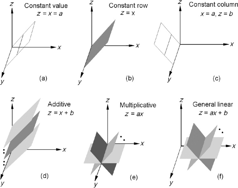
Figure 4.4 Different geometries (lines or planes) in the 3D data space for corresponding bicluster patterns. (a) A bicluster with constant values is represented by one of the lines that are parallel to the y-axis and lie in the plane x = z (the T-plane). (b) A bicluster with constant rows is represented by the T-plane. (c) A bicluster with constant columns is represented by one of the lines parallel to the y-axis. (d) A bicluster with additive coherent values is represented by one of the planes parallel to the T-plane. (e) A bicluster with multiplicative coherent values is represented by one of the planes that include the y-axis. (f) A bicluster with linear coherent values is represented by one of the planes that are parallel to the y-axis [15].
To illustrate the increased complexity of bicluster analysis compared with the traditional cluster analysis, Figure 4.5 shows the different linear bicluster patterns that are hidden in a simple 6 × 6 data matrix. Note that although we depict the biclustering problem conceptually as cutting the data matrix into submatrices as shown in Figure 4.2 (right), in fact, each bicluster requires a different permutations of the row and column indices. Hence, in general it is not possible to depict all biclusters visually in a single data matrix as in Figure 4.2 (right).
Sometime it is desirable to group data into coherent clusters based on their trends, irrespective of their actual numerical values. For this, we get bicluster patterns of coherent evolution. In this case, the data matrix consists of symbols that reflect trends in the data. The symbols can be purely nominal, of a given order, or encode positive and negative changes relative to a normal value. Figure 4.6 shows some examples of biclusters with coherent evolution. For this type of bicluster patterns, biclustering strategies different to numerical biclustering are usually used.

Figure 4.5 (a) A 6 × 6 data matrix with hidden biclusters, (b) bicluster with constant values, (c) bicluster with constant rows, (d) bicluster with constant columns, (e) bicluster of additive model, where O3 = O4 − 5 = O5 − 10 = O6 − 15 and A3 = A4 + 3 = A5 – 5 = A6 − 20, (f) bicluster of multiplicative model, where O1 = 0.2 × O6 and A5 = 0.7 × A6.
Validating the biclustering results is an important part of bicluster analysis. Biclustering results can be validated by using statistics computed from the biclusters or by using domain knowledge [12]. For example, one can compute some statistics of the biclustering solution to assess how well the biclusters found corresponding to the true biclusters in the dataset (i.e., by Jaccard Index or variants of it if ground truth is available, such as in simulated data). In many multi-objective evolutionary-based biclustering algorithms, the quality of the solutions is measured by how well the solutions meet the objectives of the algorithms, such as the homogeneity of the biclusters (i.e., by mean square residual error), size of the biclusters (bigger biclusters are preferred), or mean row variance (biclusters with larger mean row variance are assumed to be more interesting).

Figure 4.6 Types of biclusters with coherent evolution. Considering the entries of a data matrix as symbols, (a) an overall coherent evolution, (b) a coherent evolution on the rows, (c) a coherent evolution on the columns, and (d) a coherent sign change across rows.
For gene expression analysis, the preferred validation is to assess whether the biclusters found are biologically meaningful. In general, some domain knowledge about the gene expression dataset is available, and they are used to check for the biological validity of the results. A common way is to check for enrichment in the biclusters by using p-value statistics. The p-value measures the probability of including objects of a given category in a bicluster by chance. Thus, the over-represented bicluster is a bicluster of objects which is very unlikely to be obtained randomly. Currently, Gene Ontology (GO), metabolic pathway maps (MPMs), and protein–protein interaction (PPI) networks can be used to determine the biological functional relevance of genes and conditions in a bicluster. Hence, using the known gene annotation in GO, MPM, and PPI, the p-values of genes associated with the biclusters can be computed for biological validation.
4.3 BICLUSTERING TECHNIQUES
Many biclustering algorithms have been proposed recently and they can be grouped into several categories depending on the bicluster model, the search strategy, and the algorithmic framework used.
4.3.1 Distance-Based Techniques
Distance-based biclustering technique is among the earliest biclustering methods proposed in the literature. This approach measures the quality of the biclusters based on some distance metrics, and searches for the biclusters by minimizing the residual sum of squares cost. In the “direct clustering” algorithm of Hartigan [20], the sum of squares measure “SSQ” is used to evaluate the quality of each bicluster Bk = (Xk, Yk):
where ![]() is the average value in the bicluster Bk. Biclusters with lower SSQ are considered to be better than biclusters with higher SSQ. In direct clustering, the number of biclusters is fixed and the solution is reached by minimizing the sum of SSQk. Obviously, the direct clustering algorithm only searches for constant biclusters.
is the average value in the bicluster Bk. Biclusters with lower SSQ are considered to be better than biclusters with higher SSQ. In direct clustering, the number of biclusters is fixed and the solution is reached by minimizing the sum of SSQk. Obviously, the direct clustering algorithm only searches for constant biclusters.
Cheng and Church [21] were the first to introduce biclustering into gene expression data analysis. In their well-known δ-bicluster algorithm, they use the H-score, which is a mean squared residue (MSR) score, to measure the degree of coherence of a bicluster. The δ-bicluster algorithm minimizes
where aiY, aXj, and aXY are the row mean, column mean, and the mean in the submatrix B = (X, Y), respectively. It can be easily shown that Equation (4.2) is only zero for constant value, constant row or constant column, and additive bicluster patterns, but not multiplicative bicluster pattern. A bicluster is called a δ-bicluster if H(X, Y) ≤ δ for some δ > 0. To find the δ-bicluster, the score H is computed for each possible row/column addition or deletion, and the action that decreases H the most is applied. A bicluster is returned when H cannot be decreased or when H ≤ δ. After one δ-bicluster is identified, the elements in the corresponding submatrix are replaced by random numbers before finding the next δ-bicluster. The δ-biclusters are successively extracted from the raw data matrix one at a time until a prespecified number of biclusters have been identified.
Following the work of Cheng and Church, different search strategies were proposed to better detect the δ-bicluster. Bryan et al. [22] proposed a simulated annealing search technique and reported better performance on a variety of datasets. Yang et al. [23] proposed a probabilistic move-based algorithm called FLOC (FLexible Overlapped biClustering) that is able to discover multiple biclusters simultaneously. As a submatrix of a δ-bicluster is not necessarily a δ-bicluster because of outliers, Wang et al. [24] proposed the δ-pCluster model to deal with the outlier problem by further requiring that any 2 × 2 submatrix in a δ-bicluster has a pScore ≤ δ for some δ > 0, where the pScore measures the difference between elements in the 2 × 2 submatrix.
4.3.2 Factorization-Based Techniques
Factorization-based biclustering algorithm uses spectral decomposition technique to uncover “natural” substructures that are related to the main patterns of the data matrix [25, 26]. The spectral biclustering in Ref. [25] uses singular value decomposition (SVD) and assumes that the data matrix has a checkerboard structure that can be identified in eigenvectors corresponding to characteristic patterns across samples or features. Using SVD, the data matrix DN×M can be decomposed as D = U Λ VT, where Λ is a diagonal matrix with decreasing non-negative entries, and U and V are N × min(N, M) and M × min(N, M) orthonormal column matrices. If the data matrix has a block diagonal structure (with all elements outside the blocks equal to zero), then each block can be associated with a bicluster. Specifically, if the data matrix is of the form

where Di (i = 1, …, r) are arbitrary matrices, then for each Di there will be a singular vector pair (ui,vi) such that a nonzero component of ui corresponds to rows occupied by Di and a nonzero component of vi corresponds to columns occupied by Di. In a less ideal case, when the elements outside the diagonal blocks are not necessarily zeros but the diagonal blocks still contain dominating values, the SVD is able to reveal the biclusters as dominating components in the singular vector pairs.
Non-negative matrix factorization (NMF) decomposes the data as a product of two matrices that are constrained by having non-negative elements [27]. The NMF is given by D ≈ WH, where D ∈ ℜp×n is a positive data matrix with p variables and n samples, W ∈ ℜp×q are the reduced q basis vectors or factors, and H ∈ ℜq×n contains the coefficients of the linear combinations of the basis vectors needed to reconstruct the original data (also known as encoding vectors). As both the basis W and encoding vectors H are constrained to be non-negative, only additive combinations are possible. In Ref. [26], non-smooth non-negative matrix factorization algorithm (nsNMF), a variant of the NMF model, has been introduced to identify localized patterns in large datasets. In contrast to NMF, nsNMF produces sparse representation of the factors and encoding vectors by making use of non-smoothness constraints. The sparseness introduced by the algorithm produces more compact and localized feature representation of the data than the standard NMF.
4.3.3 Probabilistic-Based Techniques
The biclustering method in this category typically assumes a probabilistic model of biclusters and applies statistical parameter estimation techniques to search for biclusters [28, 29, 30, 31]. In the plaid model of Lazzeoni and Owen [30], the data matrix is viewed as consisting of a series of additive layers, that is, consisting of biclusters or subsets of rows and columns. The model first includes a background layer that accounts for the global effects in the data matrix. Then, any subsequent layer represents additional effects corresponding to biclusters of objects and features that exhibit strong pattern not explained by the background layer. The generalized plaid model is given by

where μ0 corresponds to the effect in the global background layer and θijk models the effect of layer k. The effect θijk can be expressed as a combination of μk, αik, and βjk, where μk is the background color in bicluster k, and α and β are row- and column-specific additive constants in bicluster k. The parameter ρik (or κjk) equals 1 when object i (or attribute j) belongs to layer k, and equals 0 otherwise. Any residual, not modeled by the K layers, is accounted for in the noise term ![]() ij. The biclustering process searches the layers in the dataset one after another, using the expectation maximization algorithm to estimate the model parameters until the variance of expression levels within the current layer is smaller than a threshold.
ij. The biclustering process searches the layers in the dataset one after another, using the expectation maximization algorithm to estimate the model parameters until the variance of expression levels within the current layer is smaller than a threshold.
Gu and Liu [28] proposed a fully generative model called Bayesian biclustering (BBC) algorithm for gene expression data. The data model in BBC is assumed to be

where K is the total number of clusters (unknown), μk is the main effect of cluster k, and αik and βjk are the effects of sample i and feature j, respectively, in cluster k, ![]() ijk is the noise term for cluster k, and eij models the data points that do not belong to any cluster. Here, δik = 1 indicates that sample i belongs to cluster k, and δik = 0 otherwise. Similarly, κjk = 1 indicates that feature j is in cluster k, κjk = 0 otherwise. Gibbs sampling method is used for statistical inference in BBC.
ijk is the noise term for cluster k, and eij models the data points that do not belong to any cluster. Here, δik = 1 indicates that sample i belongs to cluster k, and δik = 0 otherwise. Similarly, κjk = 1 indicates that feature j is in cluster k, κjk = 0 otherwise. Gibbs sampling method is used for statistical inference in BBC.
Sheng et al. [29] proposed a Bayesian technique for biclustering based on a simple frequency model for the expression pattern of a bicluster and on Gibbs sampling for parameter estimation. The data are discretized and every condition in a bicluster is modeled by a multinomial distribution, where the multinomial distributions for different conditions of a bicluster are assumed to be mutually independent. The Gibbs sampling sets the model in the Bayesian framework, and the Bernoulli posterior distribution is used during Gibbs sampling to find the biclusters.
4.3.4 Geometric-Based Biclustering
Based on a spatial interpretation of biclusters, a geometric-based biclustering framework has recently being introduced [15, 16, 18, 19]. The geometric viewpoint provides a unified mathematical formulation for the simultaneous detection of different types of linear biclusters (i.e., constant, additive, multiplicative, and mixed additive and multiplicative biclusters) and allows biclustering to be done with a generic plane detection algorithm.
The theoretical basis of geometric-based biclustering can be understood as follows: If we consider that the set of columns Y in B = (X, Y) spans a Y-dimensional space, then the data vector in every row of B corresponds to a point in this space. Thus, from a geometric viewpoint, the different biclusters can be considered as different linear geometric patterns in the high-dimensional data space. For example, given a matrix DN×3, a bicluster is represented by a plane in a 3D space as shown in Figure 4.7, where the N 3D samples are represented by N points. Obviously, a plane can be detected within the 3D data space which provides clues about the hidden bicluster in D. In geometric based biclustering, the problem of identification of coherent submatrices within a data matrix is formulated as the detection of linear geometric patterns (lines, planes, or hyperplanes) in a multidimensional data space [15, 19].

Figure 4.7 A plane formed by points in a bicluster in the three-dimensional data space. The gray dots are data located on the plane.
The geometric interpretation of bicluster patterns has important implication in that it unifies the commonly used linear bicluster patterns into a single linear class and allows a unified treatment in detecting these linear biclusters simultaneously. This is in contrast to most existing biclustering algorithms where the cost function implicitly imposes a constraint on the type of bicluster patterns that could be discovered. In principle, any algorithm for detecting linear geometric patterns can be employed in the geometric biclustering framework. In Refs. [15, 16, 18, 19], computer vision techniques that detect linear structures in n-dimensional space based on Hough transform have been employed to find the biclusters. This class of approach has been very successful in detecting linear bicluster patterns from a dataset and is highly robust to noise in the dataset. The major drawback is its high computation cost.
4.3.5 Biclustering for Coherent Evolution
Several biclustering algorithms that find bicluster pattern of coherent evolution have been proposed. Ben-Dor et al. [32] defined a bicluster as an order-preserving submatrix (OPSM). Specifically, a submatrix is order-preserving if there is a permutation of its columns under which the sequence of values in every row is strictly increasing. They define a complete bicluster model as the pair (Y, π) where π = (y1, …, ys) is a linear ordering of the columns in Y. A row supports (Y, π) if the s corresponding values, ordered according to the permutation π, are monotonically increasing. Since an exhaustive algorithm that tries all possible models is not feasible, the algorithm grows partial models iteratively until they become complete models. Similarly, Liu and Wang define a bicluster as an OP-Cluster (order-preserving cluster) [33] which generalizes OPSM to discover biclusters with coherent evolutions on the columns.
Murali and Kasif [34] introduced an algorithm that aims to find the largest xMOTIFs. An xMOTIF is defined as a bicluster with coherent evolutions on its rows. The data are first discretized into a set of symbols by using a list of statistically significant intervals for each row. The motifs are computed starting with a set of randomly chosen columns that act as seeds. For each column, an additional randomly chosen set A of columns is selected, called a discriminating set. The selected bicluster contains all the rows that have states equal to the seed columns and in the columns contained in the discriminating set A. The motif is discarded if less than an α-fraction of the columns matches it. After all the seeds have been used to produce xMOTIFs, the largest xMOTIF, one with the largest number of rows, is returned.
Tanay et al. [35] introduced Statistical-Algorithmic Method for Bicluster Analysis (SAMBA) to detect the biclusters of coherent evolution. The data matrix is modeled as a bipartite graph. Discovering the most significant biclusters under the weighting schemes is equivalent to the selection of the heaviest subgraphs in the bipartite graph. SAMBA assumes that each aij can be represented by two symbols S0 or S1, where S1 means change and S0 means no change. As such, the model graph has an edge between a row and a column when the object is significantly changed with the feature. A large bicluster is the one with a maximum number of rows whose symbol for aij is expected to be S1.
Prelic et al. [36] presented a fast divide-and-conquer algorithm called Bimax to detect the inclusion-maximal biclusters in the binary matrix E after a prediscretization procedure. The Bimax algorithm is similar to SAMBA. The idea behind the Bimax algorithm is to partition E into three submatrices, one of which contains only 0 cells and therefore can be disregarded in the results. The algorithm is then recursively applied to the remaining two submatrices U and V. The recursion ends if the current matrix represents a bicluster, that is, contains only 1s. If U and V do not share any rows and columns of E, the two matrices can be processed independently from each other. However, if U and V have a set, X, of rows in common, special care is necessary to only generate those biclusters in V that share at least one common column with X. Uitert et al. [37] proposed BicBin (Biclustering Binary data) to find a contiguous block for a large, binary, and sparse genomic data matrix, such as transcription factor binding site, insertional mutagenesis, and gene expression. Assuming that each element in D is the outcome of a Bernoulli trial, a probability-based score function is derived in BicBin to evaluate a submatrix.
4.4 EVOLUTIONARY ALGORITHMS BASED BICLUSTERING
Evolutionary algorithm is a meta-heuristic technique that has been successfully used for various optimization problems because of its excellent exploratory capability in a global search space and its good ability to solve complex problems [38, 39]. Hence, many biclustering algorithms that utilize the EA framework as a search strategy have been proposed. There are two main EA frameworks; the first is based on the genetic algorithm (GA), and the second is based on the artificial immune system (AIS).
Genetic algorithms are a class of EAs which generate solutions to optimization problems using techniques inspired by natural evolution, such as inheritance, mutation, selection, and crossover. In a GA, a population of candidate solutions, called individuals, to an optimization problem is evolved toward better solutions over several generations. Each candidate solution has a set of properties encoded as a chromosome that can be mutated and altered during iteration to form the next generation.
In GA-based biclustering of gene expression data, the row and column indices of the data matrix that correspond to a solution for a bicluster are encoded in a chromosome. The chromosome encoding usually consists of two parts; the first part consists of bit string for genes, and the second part consists of bit string for conditions. For fixed length chromosome, the length of bit string for genes equals the number of rows in the gene expression data matrix, and the length of bit string for conditions equals the number of columns. A bit is set to 1 if the corresponding gene and/or condition is present in the bicluster, and 0 otherwise. At each iteration, the operations of cross-over and mutation are performed to generate the offspring population, and the parent and offspring populations are combined in a pool from which the next generation is selected based on fitness of the individuals.
Artificial immune systems are a class of computationally intelligent systems inspired by the principles and processes of the biological immune system. Depending on the specific immunological theories that AIS is inspired by, the techniques used in AIS can be classified into three types: clonal selection, negative selection, and immune network.
The clonal selection algorithms are inspired by the antigen-driven affinity maturation process of B-cells, with its associated hypermutation mechanism. During the clonal expansion of B-cells, the average antibody affinity increases for the antigen that triggered the clonal expansion. This phenomenon is called affinity maturation, and is responsible for the fact that upon a subsequent exposure to the antigen, the immune response is more effective due to the antibodies having a higher affinity for the antigen. Affinity maturation is caused by a somatic hypermutation and the selection mechanism that occurs during the clonal expansion of B-cells. Somatic hypermutation alters the specificity of antibodies by introducing random changes to the genes that encode for them.
Castro and Zuben [40] proposed a clonal selection algorithm named “CLONALG” for optimization. Two important features of affinity maturation in B-cells are exploited in CLONALG. The first is that the proliferation of B-cells is proportional to the affinity of the antigen that binds it, thus the higher the affinity, the more the clones are produced. Second, the mutations suffered by the antibody of a B-cell are inversely proportional to the affinity of the antigen it binds. CLONALG generates a population of N antibodies, each specifying a random solution for the optimization process. During each iteration, a subset of the best antibodies with the highest affinity to the antigens is selected, cloned, and mutated in order to construct a new candidate population. Finally, a percentage of worst antibodies of previous generation are replaced with new randomly create ones.
Negative selection algorithms are inspired by the main mechanism in the thymus that produces a set of mature T-cells capable of binding only non-self antigens. The process of deleting self-reactive lymphocytes is termed clonal deletion and is carried out via a mechanism called negative selection that operates on lymphocytes during their maturation. For T-cells this mainly occurs in the thymus, which provides an environment rich in antigen presenting cells that present self-antigens. Immature T-cells that strongly bind these self-antigens undergo apoptosis. Thus, the T-cells that survive this process should be unreactive to self-antigens. The property of lymphocytes not to react with the self is called immunological tolerance. The first negative selection algorithm was proposed by Forrest et al. [41] to detect data manipulation caused by a virus in a computer system. The starting point of this algorithm is to produce a set of self-strings S that define the normal state of the system. The task then is to generate a set of detectors D that only bind/recognize the complement of S. These detectors can then be applied to new data in order to classify them as being self or non-self, or whether they have been manipulated.
In the immune network theory [42], in the absence of foreign antigen, the immune system displays behavior or activity resulting from interactions with itself, and from these interactions immunological behavior such as tolerance and memory emerge. The immune network algorithms focus on the network graph structures involved where antibodies (or antibody-producing cells) represent the nodes and the training algorithm involves growing or pruning edges between the nodes based on affinity. Immune network algorithms have been used in clustering, data visualization, control, and optimization domains, and share properties with artificial neural networks [43].
In Ref. [44], a multi-objective GA biclustering algorithm using non-dominated sorting genetic algorithm (NSGA-II) was proposed. In multi-objective optimization [45], the objective function or fitness function consists of two or more conflicting objectives. A solution, which is better with respect to one objective, requires a compromise in other objectives. Hence, there is no single optimum solution. Rather, there exists a set of solutions that are all optimal involving tradeoffs between conflicting objectives. In multi-objective optimization, the set of optimal solution constitute the Pareto front. A solution belongs to the Pareto front (or is Pareto optimal) if there is no other feasible solution capable of reducing the value of one objective without simultaneously increasing at least one of the others. These solutions are called non-dominating. To obtain Pareto optimal solutions that are well spaced out on the Pareto front, that is, with good diversity, the concept of crowding is used. The idea is to retain solutions that are far apart from each other. NSGA-II [46] has three main properties—non-domination, crowding distance, and crowding selection operator—that implement these concepts. In Ref. [44], a local search mechanism, based on the node insertion and deletion heuristics proposed by Cheng and Church [21], was added into NSGA-II. The algorithm employs a binary encoding representation, where each individual in the population is a binary vector with a size equal to the number of rows plus the number of columns of the dataset. A value of 1 in the vector indicates that the corresponding row or column is present in the bicluster. The algorithm starts with a given bicluster. The irrelevant genes or conditions having MSR above (or below) a certain threshold are then selectively eliminated (or added) to the bicluster. Finally, the nodes with low contribution to the residue are added back to the bicluster to increase the volume of the bicluster as long as the residue is smaller than a predefined threshold. These node deletion and insertion procedures are basically greedy procedures similar to Cheng and Church's algorithm. The algorithm uses standard GA operators for crossover and mutation, that is, single-point crossover, single bit mutation, to generate the next generation. Both statistical and biological validations were performed to verify the biclustering results.
In Ref. [47], a multi-objective GA biclustering algorithm which has three objectives and uses NSGA-II optimization with local search based on Cheng and Church's heuristics was proposed. The first objective is the size of the bicluster, the second objective is the MSR score of Cheng and Church, and the third objective is the mean row variance Rvar(I,J) given by
Note that maximizing Rvar(I,J) tends to find biclusters with genes that exhibit significant fluctuations in the different conditions, that is, biclusters with significant row variances. Hence, even though both constant value bicluster and additive model bicluster will minimize MSR, only the later maximizes Rvar(I,J). The encoding used in this algorithm is based on representing a bicluster as a string composed of two parts: the first part is an ordered row index and the second part is an ordered column index. Single point crossover operator is used in each part of the solution (row part and column part), and each part undergoes crossover separately by exchanging index lists of the two parents after the crossover points obtained as follows. Let the two parents be P1 = {r1…rn c1…cm} and P2 = {r′1…r′lc′1…c′k}, where rn ![]() r′l. The row part crossover point in P1 is generated as a random integer in the range 2
r′l. The row part crossover point in P1 is generated as a random integer in the range 2 ![]() λ1
λ1 ![]() rn, then the crossover point in P2 is obtained by λ2 = r′j where r′j ⩾ λ1 and r′j − 1
rn, then the crossover point in P2 is obtained by λ2 = r′j where r′j ⩾ λ1 and r′j − 1 ![]() λ1. Similarly, the column part crossover points are obtained. For the mutation operator, instead of random mutation as in conventional GA, a local search based on Cheng and Church's heuristics is used. Only statistical validation was done to validate the biclustering results.
λ1. Similarly, the column part crossover points are obtained. For the mutation operator, instead of random mutation as in conventional GA, a local search based on Cheng and Church's heuristics is used. Only statistical validation was done to validate the biclustering results.
In Ref. [48], a multi-objective GA biclustering algorithm called “MOGAB” was proposed. MOGAB uses a variable length string that encodes the A gene clusters and B condition clusters to represent the A×B biclusters. It finds biclusters with high mean row variance and an MSR below a threshold δ by optimizing a two-objective function based on the NSGA-II algorithm. MOGAB uses simple single-point crossover, where the gene part and the condition part of the string undergo crossover separately. For the gene part, two crossover points are chosen on the two parent chromosomes, respectively, and the portions of the chromosomes beyond these crossover points are exchanged. Similarly, the crossover for the condition part is performed. Single bit mutation for the gene part and condition part is performed by replacing a randomly chosen position in that part with another randomly chosen index from the corresponding part, respectively. The biclustering results were validated both statistically and biologically.
In Ref. [49], a GA-based multi-objective biclustering algorithm that identifies fuzzy biclusters was introduced. Instead of crisp assignment, fuzzy assignment of genes and conditions was done by using the membership and medoid updating rules adopted from the fuzzy c-mediods algorithm. The biclustering algorithm optimizes three objectives: fuzzy bicluster volume, fuzzy MSR, and fuzzy mean row variance. This algorithm uses a string encoding consisting of a gene part and a condition part, where the indices in each part consist of indices of genes or conditions that act as cluster medoids of genes or conditions. NSGA-II optimization algorithm was used to find the biclusters. Standard GA operators for crossover and mutation, that is, single-point crossover and single bit mutation, were used to generate the next generation. Only statistical validation was used to validate the biclustering results.
In Ref. [50], a multi-objective multi-population artificial immune network (MOM-aiNet) was proposed to detect additive biclusters. The two objectives used in MOM-aiNet are MSR and bicluster volume. These objectives constitute the affinity function that selects the non-dominated individuals in the subpopulation. The algorithm starts with the generation of n subpopulations of one bicluster each, generated by randomly choosing one row and one column of the dataset. Then in the main loop, cloning of each subpopulation occurs, followed by mutation. In the mutation process, each clone undergoes one of the three possible actions, that is, insert a row, insert a column, and remove a row or column, with equal probability. After mutation, all the non-dominated biclusters of this subpopulation (consisting of the original individuals and the mutated clones) are selected to generate the new subpopulation for the next iteration. As each of these subpopulations is cloned and mutated, they converge to distinct promising regions of the search space. MOM-aiNet also performs a suppression operation from time to time, by comparing the degree of overlap of the largest biclusters of each subpopulation. If the overlap is over a set threshold, the two subpopulations are merged into a single subpopulation, and the non-dominated individuals are selective from this new subpopulation. To promote diversity and explore new regions of the search space, random insertion of new subpopulations is also performed from time to time.
One feature of MOM-aiNet is that it keeps not only the best individual of each sub-population, but also several locally (within their subpopulation) non-dominated ones at each generation. The final result returned by MON-aiNet includes not only the final set of non-dominated (i.e., Pareto optimal) individuals, but also all the non-dominated individuals within each subpopulation. Hence, the final set of solutions may provide a higher coverage of the data matrix but may also contain suboptimal biclusters that capture important correlations in the data. The biclustering results on two gene expression datasets and a MovieLens dataset are evaluated based on statistical measures such as MSR, bicluster volume, Pareto front coverage, and overlap. It was shown that MOM-aiNet could provide biclustering solution that maximizes the coverage of the data while minimizing overlap, mainly because of its multi-population aspect and its suppression mechanism, which inhibits two subpopulations from exploring similar areas of the search space.
In Ref. [51], we introduced a technique called condition-based evolutionary biclustering (CBEB) algorithm based on HC and EA search. The general framework of the algorithm is as follows: to search for biclusters in a subspace of conditions, an EA + HC search strategy is used. The chromosome of an individual in the EA method encodes the indices of the conditions in each subspace. All of the rows and the columns corresponding to the selected indices in the chromosome form a submatrix. The conventional HC algorithm is then applied to the submatrix. The clusters in the submatrix obtained from HC can be considered as biclusters in the subspace. Since a bicluster discovered from a single subspace may be a part of a larger bicluster crossing multiple subspaces, after the biclusters are found in each subspace, an expand-and-merge operation is performed to obtain the final biclustering output. The biclustering result obtained from the EA + HC procedure is finally verified using an MSR-based fitness function. As the column dimension of the gene expression data matrix is divided into a number of subsets and EA computation is performed in parallel in each of these subspaces, high computation cost of performing EA search in a space created by a large number of experimental conditions is avoided.
In CBEB, binary encoding is chosen, and each individual (solution) represents one binary chromosome with the bit string length, the same as the column number of the corresponding subspace. For each individual in the population, a bit equal to 1 indicates that the corresponding column is selected to form a submatrix Ms. Ms contains full rows from the original data matrix. Once the submatrix is formed, HC is performed to detect biclusters in this submatrix. The fitness of the solution is evaluated based on a criterion that favors the solution with smaller MSR score and larger bicluster numbers. Solutions with better fitness survive to the next generation and can reproduce offspring. In this work, we employed both the simple crossover method and the binary mutation method for reproducing the offspring. Once EA-based search of the optimal subspaces is performed and a set of biclusters Bic_Set is obtained, we first expand each bicluster in Bic_Set and then merge small biclusters into larger ones. In expanding the biclusters, a new column is added into a specific bicluster if the newly formed bicluster satisfies the MSR score with a predefined threshold. Similarly, a row is added to the bicluster if the newly expanded bicluster meets the same criterion. In merging biclusters, a smaller bicluster can be merged into a larger one if they mostly overlap.
The CBEB algorithm is evaluated using synthetic data based on the matching score S. Given two sets of biclusters, M1 and M2, the match score of M1 with respect to M2 is formulated as
where B(I, J) denotes a bicluster with the set of rows (I) and the set of columns (J). Let Mop denote the best set of biclusters and Mt the set of biclusters to be evaluated. The S(Mop,Mt) can represent the quality of the biclusters in Mt with respect to the best biclusters in Mop. For real dataset, the quality of the biclusters is evaluated based on statistical enrichment using GO. Experiments indicated that CBEB significantly outperformed several popular biclustering algorithms on both the synthetic and real datasets. Figure 4.8 shows the result of a comparative study of seven algorithms on the S. cerevisiae gene expression dataset from [52].
Note that all the algorithms discussed above detect biclusters with homogeneity defined by the MSR score. It is easy to show that while the MSR for a perfect additive bicluster is 0, it is not true for multiplicative bicluster patterns. As MSR score can only detect additive bicluster patterns, these algorithms are, in principle, only capable of detecting additive bicluster patterns. Additive bicluster patterns are sometime called shifting patterns since the rows or columns in a bicluster are “shift” of other rows or columns in the bicluster.
In order to handle multiplicative biclusters, which are sometime called scaling patterns, Giraldez et al. [53] introduced the maximal standard area (MSA) as another homogeneity criterion besides the MSR in their multi-objective GA biclustering algorithm called sequential multi-objective biclustering (SMOB). The MSA basically measures the area bounded by the maximum and minimum values of standardized expression levels of genes within a bicluster and could handle the non-parallel shifting pattern to some extent as seen in the multiplicative bicluster pattern. SMOB detects biclusters by optimizing four objectives: size of bicluster, MSR, mean row variance, and MSA. Note that although SMOB was able to detect some multiplicative biclusters due to the use of MSA, the MSA does not actually model multiplicative patterns. Noise in the data would create non-parallel shifting patterns, even if the true bicluster pattern is additive. As MSA is not a model for multiplicative bicluster patterns, there is no guarantee that it will find all multiplicative biclusters. A similar attempt to handle both additive and multiplicative bicluster patterns based on data standardization is proposed by Pontes et al. [54] in their algorithm called Evo-Bexpa. In this algorithm, the expression values are standardized by


Figure 4.8 Proportion of biclusters significantly enriched by Gene Ontology biological process for different algorithms, where α is the adjusted significant level for the biclusters.
where μcj and σcj are the mean and the standard deviation of column j, respectively. Similar to MSA, the standardization only reduces the column variations (i.e., to 0 mean and 1 standard deviation) but does not actually model multiplicative bicluster patterns. Nevertheless, the standardization scales down the column variations such that multiplicative patterns are more likely to satisfy the MSR score commonly used in many biclustering algorithms.
In Ref. [15, 19], we proposed a class of geometric-based biclustering algorithms that could detect biclusters with general linear patterns. As both additive and multiplicative patterns are the special cases of linear patterns, our algorithms were able to simultaneously detect all additive and multiplicative biclusters. In our approach, a linear bicluster is viewed as a hyperplane in a high-dimensional space. For a submatrix (R, C), a linear bicluster satisfies

where u1, u2, …, u|C|, v ∈ ℜ and at least one of the ui is nonzero, and |C| is the cardinality of the column set C. The set of all genes x = (x1, x2, …, x|C|)T that satisfy Equation (4.9) is called a hyperplane of the space ℜ|C|. In Figure 4.9, all genes {x1, x2, x3, x4, x5} are on the same hyperplane whose equation is given by c1 = 0.5c2 – 1.5c3 + 2c4 + 3c5 – c6.
x1 x2 x3 x4 x5 Figure 4.9 Graphical representation of a bicluster containing linear patterns whose relationship is c1 = 0.5c2 – 1.5c3 + 2c4 + 3c5 – c6 as shown in the table above.
c1
c2
c3
c4
c5
c6
0.55
1
2.5
3
0.6
4
4.95
2.5
3
1.5
2
0.8
8.75
0.8
0.9
0.6
3
0.5
5.55
1.2
1.5
1.6
2.1
2.3
7.95
4.5
2.2
3.1
1.2
0.8

In Ref. [17], we proposed to detect linear biclusters by searching for hyperplanes using GA. Given a gene a = (a1, a2, …, a|C|)T and a hyperplane H = {x ∈ R|C|: uTx = v}, the distance from a to H is given by

In biclustering, we need to find the hyperplane that minimizes the total distances from the hyperplane to all genes in the bicluster. Therefore, the problem for biclustering is formulated as the following GA optimization problem:
Find z = (u1, u2, …, u|C|, v)T and a submatrix (G, C) ⊆ A which minimizes

subject to

The above optimization problem is a mixture of discrete and continuous search spaces because the domains of hyperplane parameters and submatrix are continuous and discrete spaces, respectively. We employed GA to find the biclusters. Our algorithm is shown in Figure 4.10.
In our algorithm, each individual which has a dynamic set of biclusters (R, C) is represented by integer string encoding. More specifically, each individual has two subsets containing selected rows and columns and separated by zero values. Figure 4.11 is an illustration of this encoding with three biclusters, and the sets of rows and columns of the first bicluster are {3, 2, 5} and {1, 8}, respectively.
Figure 4.10 Pseudo-code of linear biclusters detection based on the genetic algorithm.

Figure 4.11 Individual chromosome encoding.
The parameters of evolutionary computation listed in Table 4.1 are chosen experimentally and the fitness function of each individual is given by

where h is number of biclusters in an individual. In step 2, the iteration of the steepest descent method is stopped if the number of iterations reaches a predefined number or if there are negligible changes in fitness function values between two consecutive iterations.
To validate our algorithm, we run it on simulated datasets where ground truth is known and also on real gene expression datasets. Our algorithm was compared with six other biclustering algorithms, namely FABIA [55], ISA2 [56], xMOTIF [34], Cheng and Church [21], spectral biclustering [25], plaid model [30]. For the simulated datasets, we performed 100 runs by randomly generated 100 datasets whose sizes are 200 rows by 40 columns. Four biclusters of linear model with the number of rows and columns randomly selected within the range from 20 to 40 and 7 to 15, respectively, were embedded into each of these datasets. The Jaccard coefficient was used to measure the similarity between the two biclusters:

where G1 and G2 are two biclusters. The higher the Jaccard index, the better the performance of the algorithm.
The Jaccard index was computed from the results and the mean and standard deviation of the Jaccard indices over 100 runs are listed in Table 4.2. Note that xMOTIF and spectral biclustering could not find any of the linear biclusters. Our algorithm performed the best with the highest mean Jaccard index and the smallest standard deviation values over the 100 runs among all compared algorithms.
Table 4.1 Parameters of genetic algorithm
| Parameter | Value |
| Population size | 500 |
| Number of generations | 20 |
| Probability of reproduction | 0.1 |
| Probability of crossover | 0.7 |
| Probability of mutation | 0.2 |
Table 4.2 Average Jaccard index based on 100 simulated datasets
| Methods | Mean | Standard deviation |
| The proposed algorithm | 0.4848 | 0.0264 |
| xMOTIF | N/A | N/A |
| Spectral biclustering | N/A | N/A |
| Plaid model | 0.0329 | 0.1156 |
| Cheng and Church | 0.0333 | 0.0707 |
| ISA2 | 0.1667 | 0.3430 |
| FABIA | 0.0036 | 0.0226 |
We tested our algorithm on the gene expression dataset of diffuse large B-cell lymphoma [57]. The diffuse large-B-cell lymphoma was used to predict the survival after chemotherapy and contains 180 samples of 661 genes. To evaluate the biclustering results, we used GO-TermFinder [58] and ClueGO [59] to assess the biological relevance of the biclusters based on the GO [60] and Kyoto Encyclopedia of Genes and Genomes (KEGG) pathway [61] annotations. All biclusters obtained from biclustering algorithms were enriched to three GO categories: GO biological process (GO BP), GO molecular function (GO MF), GO cellular component (GO CC), and the KEGG pathway. The number of biclusters found by our algorithm and six other biclustering algorithms enriched by three GO categories and KEGG pathway are shown in Tables 4.3, 4.4, 4.5, 4.6, and 4.7. For this dataset, xMOTIF did not give any bicluster, and Cheng and Church considered the whole dataset as a bicluster, while spectral clustering and plaid model gave only one bicluster that was not significantly enriched by the three GO categories and KEGG pathway.
Table 4.3 Number of biclusters found
| Methods | Number of biclusters |
| The proposed algorithm | 13 |
| xMOTIF | 0 |
| Spectral biclustering | 1 |
| Plaid model | 1 |
| Cheng and Church | 1 |
| ISA2 | 10 |
| FABIA | 5 |
Table 4.4 Number of biclusters enriched by GO BP
| Methods | p-value = 0.05 | p-value = 0.01 |
| The proposed algorithm | 13 | 13 |
| xMOTIF | 0 | 0 |
| Spectral biclustering | 0 | 0 |
| Plaid model | 0 | 0 |
| Cheng and Church | 1 | 1 |
| ISA2 | 8 | 7 |
| FABIA | 5 | 5 |
GO BP, GO biological process.
Table 4.5 Number of biclusters enriched by GO MF
| Methods | p = 0.05 | p = 0.01 |
| The proposed algorithm | 13 | 13 |
| xMOTIF | 0 | 0 |
| Spectral biclustering | 0 | 0 |
| Plaid model | 0 | 0 |
| Cheng and Church | 1 | 1 |
| ISA2 | 2 | 2 |
| FABIA | 3 | 3 |
GO MF, GO molecular function.
Table 4.6 Number of biclusters enriched by GO CC
| Methods | p = 0.05 | p = 0.01 |
| The proposed algorithm | 12 | 11 |
| xMOTIF | 0 | 0 |
| Spectral biclustering | 0 | 0 |
| Plaid model | 0 | 0 |
| Cheng and Church | 1 | 1 |
| ISA2 | 5 | 3 |
| FABIA | 3 | 1 |
GO CC, GO cellular component.
Table 4.7 Number of biclusters enriched by KEGG pathway
| Methods | p = 0.05 | p = 0.01 |
| The proposed algorithm | 13 | 10 |
| xMOTIF | 0 | 0 |
| Spectral biclustering | 0 | 0 |
| Plaid model | 0 | 0 |
| Cheng and Church | 1 | 1 |
| ISA2 | 5 | 5 |
| FABIA | 4 | 3 |
KEGG, Kyoto Encyclopedia of Genes and Genomes.
4.5 CONCLUSION
Bicluster analysis has recently emerged as a powerful tool for unsupervised pattern discovery, especially for the analysis of gene expression data. However, biclustering is an NP-hard problem, and there is a need for highly effective and efficient search algorithms to find the biclusters in the dataset. Evolutionary algorithms have generated a lot of interest in the optimization community due to its ability to find near optimal solution in many hard optimization problems. In this chapter, we provided a comprehensive review of the biclustering of gene expression data and the application of EAs to solve the biclustering problem. We first described the different types of bicluster patterns and highlighted an interesting and important viewpoint of the biclustering problem: the detection of linear hyperplanes in a high-dimensional data space. As different types of algorithms have been proposed for gene expression data biclustering depending on the objective functions, search strategies, and algorithmic frameworks used, we also briefly described some representative algorithms in each category. We reviewed recent application of GAs and artificial immunity system algorithms to the biclustering problem and presented some of our own results. To handle multiple (possibly conflicting) objectives in the optimization, many of these EAs employ the concept of Pareto optimality and search for a set of solutions, called non-dominating solutions, that constitute the Pareto front. We stressed that the majority of these evolutionary biclustering algorithms detect only the additive bicluster pattern and there is a need for algorithms that can handle the more general linear bicluster pattern.
REFERENCES
- D. A. Rew, “DNA microarray technology in cancer research”, European Journal of Surgical Oncology, 27(5): 504–508, 2001.
- T. R. Golub, et al., “Molecular classification of cancer: class discovery and class prediction by gene expression monitoring”, Science, 286(5439): 531–537, 1999.
- P. D'haeseleer, S. Liang, R. Somogyi, “Genetic network inference: from co-expression clustering to reverse engineering”, Bioinformatics, 16(8): 707–726, 2000.
- M. T. Laub, H. H. McAdams, T. Feldblyum, C. M. Fraser, L. Shapiro, “Global analysis of the genetic network controlling a bacterial cell cycle”, Science, 290(5499): 2144–2148, 2000.
- J. L. DeRisi, V. R. Iyer, P. O. Brown, “Exploring the metabolic and genetic control of gene expression on a genomic scale”, Science, 278(5338): 680–686, 1997.
- S. Tavazoie, J. D. Hughes, M. J. Campbell, R. J. Cho, G. M. Church, “Systematic determination of genetic network architecture”, Nature Genetics, 22(3): 281–285, 1999.
- M. B. Eisen, P. T. Spellman, P. O. Brown, D. Botstein, “Cluster analysis and display of genome-wide expression patterns”, Proceedings of the National Academy of Sciences of the United States of America, 95(25): 14863–14868, 1998.
- P. Tamayo, D. Slonim, J. Mesirov, Q. Zhu, S. Kitareewan, E. Dmitrovsky, E. S. Lander, T. R. Golub, “Interpreting patterns of gene expression with self-organizing maps: methods and application to hematopoietic differentiation”, Proceedings of the National Academy of Sciences of the United States of America, 96(6): 2907–2912, 1999.
- D. Reiss, N. Baliga, R. Bonneau, “Integrated biclustering of heterogeneous genome-wide datasets for the inference of global regulatory networks”, BMC Bioinformatics, 7(1): 280, 2006.
- S. Busygin, O. Prokopyev, P. M. Pardalos, “Biclustering in Data Mining”, Computers and Operation Research, 35: 2964–2987, 2008.
- S. C. Madeira, A. L. Oliveira. Biclustering algorithms for biological data analysis: a survey. IEEE/ACM Transactions on Computational Biology and Bioinformatics, 1: 24–45, 2004.
- H. Zhao, A. W. C. Liew, D. Z. Wang, H. Yan, “Biclustering analysis for pattern discovery: current techniques, comparative studies and applications”, Current Bioinformatics, 7(1): 43–55, 2012.
- A. W. C. Liew, N. F. Law, H. Yan, “Recent Patents on Biclustering Algorithms for Gene Expression Data Analysis”, Recent Patents on DNA and Gene Sequences, 5(2): 117–125, 2011.
- K. O. Cheng, N. F. Law, W. C. Siu, A. W. C. Liew, “Identification of coherent patterns in gene expression data using an efficient biclustering algorithm and parallel coordinate visualization”, BMC Bioinformatics, 9: 210, 2008.
- X. Gan, A. W. C. Liew, H. Yan, “Discovering biclusters in gene expression data based on high-dimensional linear geometries”, BMC Bioinformatics, 9: 209, 2008.
- H. Zhao, A. W. C. Liew, X. Xie, H. Yan, “A new geometric biclustering algorithm based on the Hough transform for analysis of large-scale microarray data”, Journal of Theoretical Biology, 251(2): 264–274, 2008.
- C. To, A. W. C. Liew, “Genetic algorithm based detection of general linear biclusters”, 2014 International Conference on Machine Learning and Cybernetics, ICMLC2014, Lanzhou, China, July 13–16, 2014.
- H. Zhao, A. W. C. Liew, H. Yan, “A new strategy of geometrical biclustering for microarray data analysis” Proceedings of the Fifth Asia Pacific Bioinformatics Conference, APBC2007, Hong Kong, January 15–17, pp. 47–56, 2007.
- X. Gan, A. W. C. Liew, H. Yan, “Biclustering gene expression data based on a high dimensional geometric method”, Proceedings of the Fourth International Conference on Machine Learning and Cybernetics (ICMLC 2005), Guangzhou, China, August 18–21, 2005.
- J. A. Hartigan, “Direct clustering of a data matrix”, Journal of the American Statistical Association, 67(337): 123–129, 1972.
- Y. Cheng, G. M. Church, “Biclustering of expression data”, Proceedings of 8th International Conference on Intelligent Systems for Molecular Biology, Menlo Park, CA, pp. 93–103, 2000.
- K. Bryan, P. Cunningham, N. Bolshakova, “Biclustering of expression data using simulated annealing”, Proceedings of the 18th IEEE Symposium on Computer-Based Medical Systems, Washington, DC, pp. 383–388, 2005.
- J. Yang, W. Wang, H. Wang, P. Yu, “Enhanced biclustering on expression data”, Proceedings of the Third IEEE Conference Bioinform Bioeng, Bethesda, Maryland, pp. 321–327, 2003.
- H. Wang, W. Wang, J. Yang, P. Yu, “Clustering by pattern similarity in large data sets”, Proceedings of the 2002 ACM SIGMOD Int'l Conference Management of Data, Madison, Wisconsin, pp. 394–405, 2002.
- Y. Klugar, R. Basr, J. T. Chang, M. Gerstein, “Spectral biclustering of microarray data: Coclustering genes and conditions”, Genome Research, 13: 703–716, 2003.
- P. Carmonan-Saez, R. D. Pascual-Marqui, F. Tirado, J. M. Carazo, A. Pascual-Montano, “Biclusteing of gene expression data by non-smooth non-negative matrix factorization”, BMC Bioinformatics, 7: 78, 2006.
- D. D. Lee, H. S. Seung, “Learning the parts of objects by nonnegative matrix factorization”, Nature, 401: 788–791, 1999.
- J. Gu, J. S. Liu, “Bayesian biclustering of gene expression data”, BMC Genomics, 9: 4, 2008.
- Q. Sheng, Y. Moreau, B. De Moor, “Biclustering microarray data by Gibbs sampling”, Bioinformatics, 19: ii196–ii205, 2003.
- L. Lazzeroni, A. Owen, “Plaid models for gene expression data”, Technical report, Stanford University, Stanford, CA, 2000.
- G. Govaert, M. Nadif, “Clustering with block mixture models”, Pattern Recognition, 36(2): 463–473, 2003.
- A. Ben-Dor, B. Chor, R. Karp, Z. Yakhini, “Discovering local structure in gene expression data: The order-preserving submatrix problem”, Journal of Computational Biology, 10(3–4): 373–384, 2003.
- J. Liu, W. Wang, “OP-Cluster: Clustering by tendency in high dimensional space”, Proceedings of the 3rd IEEE Int’l Conference Data Mining, Florida, USA, pp. 187–194, 2003.
- T. M. Murali, S. Kasif, “Extracting conserved gene expression motifs from gene expression data”, Proceedings of Pacific Symposium on Biocomputing, Lihue, Hawaii, 8: 77–88, 2003.
- A. Tanay, R. Sharan, R. Shamir, “Discovering statistically significant biclusters in gene expression data”, Bioinformatics, 18: S136–S144, 2002.
- A. Prelic, et al., “A systematic comparison and evaluation of biclustering methods for gene expression data”, Bioinformatics, 22: 1122–1129, 2006.
- M. Uitert, W. Meuleman, L. Wessels, “Biclustering sparse binary genomic data”, Journal of Comparative Biology, 15(10): 1329–1345, 2008.
- M. Mitchell. An Introduction to Genetic Algorithm, MIT Press, London, 2001.
- K. A. De Jong, Evolutionary Computation: a Unified Approach, MIT Press, Cambridge, MA, 2006.
- L. N. de Castro, F. J. Von Zuben, “Learning and optimization using the clonal selection principle”, IEEE Transactions on Evolutionary Computation, Special Issue on Artificial Immune Systems, 6(3): 239–251, 2002.
- S. Forrest, A. S. Perelson, L. Allen, R. Cherukuri, “Self-Nonself discrimination in a computer”, Proceedings of IEEE Symposium on Research in Security and Privacy, Oakland, CA, pp. 202–212, 1994.
- N. K. Jerne, “Towards a network theory of the immune system”, Annals of Immunology, 125C: 373–389, 1974.
- J. Timmis, M. Neal, J. Hunt, “An artificial immune system for data analysis”, Biosystems, 55(1): 143–150, 2000.
- S. Mitra, H. Banka, “Multi-objective evolutionary biclustering of gene expression data”, Pattern Recognition, 39: 2464–2477, 2006.
- K. Deb, Multi-Objective Optimization Using Evolutionary Algorithms. Wiley, London, 2001.
- K. Deb, A. Pratap, S. Agarwal, T. Meyarivan, “A fast and elitist multiobjective genetic algorithm: NSGA-II”, IEEE Transactions on Evolutionary Computation, 6(2): 182–197, 2002.
- K. Seridi, L. Jourdan, E. Talbi, “Multi-objective evolutionary algorithm for biclustering in microarrays data”, Proceeding of IEEE Congress on Evolutionary Computation, New Orleans, USA, pp. 2593–2599, 2011.
- U. Maulik, S. Bandyopadhyay, “Finding multiple coherent biclusters in microarray data using variable string length multi-objective genetic algorithm”, IEEE Transactions on Information Technology in Biomedicine, 13: 969–975, 2009.
- U. Maulik, A. Mukhopadhyay, S. Bandyopadhyay, M. Q. Zhang, X. Zhang, “Multiobjective fuzzy biclustering in microarray data: method and a new performance measure”, Proceedings of the IEEE Congress on Evolutionary Computation, Hong Kong, 2008, pp. 1536–1543,.
- G. P. Coelho, F. O. de Franca, F. J. Von Zuben, “Multi-objective biclustering: when non-dominated solutions are not enough”, Journal of Mathematical Modelling and Algorithms, 8: 175–202, 2009.
- Q. Huang, D. Tao, X. Li, A. W. C. Liew, “Parallelized evolutionary learning for detection of biclusters in gene expression data”, IEEE/ACM Transactions on Computational Biology and Bioinformatics, 9:560–570, 2012.
- A. P. Gasch, P. T. Spellman, C. M. Kao, O. Carmel-Harel, M. B. Eisen, G. Storz, D. Botstein, P. O. Brown, “Genomic expression programs in the response of yeast cells to environmental changes”, Molecular Biology of the Cell, 11: 4241–4257, 2000.
- R. Giraldez, F. Divina, B. Pontes, J. S. Aguilar-Ruiz, “Evolutionary search of biclusters by minimal intrafluctuation”, Proceedings of the IEEE International Fuzzy Systems Conference, London, UK, pp. 1–6, 2007.
- B. Pontes, R. Giraldez, J. S. Aguilar-Ruiz, “Configurable pattern-based evolutionary biclustering of gene expression data”, Algorithms for Molecular Biology, 8: 4, 2013.
- S. Hochreiter, U. Bodenhofer, M. Heusel, A. Mayr, A. Mitterecker, A. Kasim, T. Khamiakova, S. Van Sanden, D. Lin, W. Talloen, L. Bijnens, H. W. Göhlmann, Z. Shkedy, D. A. Clevert, “FABIA: factor analysis for bicluster acquisition”, Bioinformatics, 26: 1520–1527, 2010.
- J. Ihmels, S. Bergmann, N. Barkai, “Defining transcription modules using large-scale gene expression data”, Bioinformatics, 20: 1993–2003, 2004.
- A. Rosenwald, et al., “The use of molecular profiling to predict survival after chemotherapy for diffuse large-B-cell lymphoma”, New England Journal of Medicine, 346: 1937–1947, 2002.
- E. I. Boyle, S. Weng, J. Gollub, H. Jin, D. Botstein, J. M. Cherry, G. Sherlock, “GO: TermFinder—open source software for accessing Gene Ontology information and finding significantly enriched Gene Ontology terms associated with a list of genes”, Bioinformatics, 20: 3710–3715, 2004.
- G. Bindea, et al., ClueGO: a Cytoscape plug-in to decipher functionally grouped gene ontology and pathway annotation networks”, Bioinformatics, 25: 1091–1093, 2009.
- M. Ashburner, et al., “Gene Ontology: tool for the unification of biology”, Nature Genetics, 25: 25–29, 2000.
- M. Kanehisa, S. Goto, “KEGG: kyoto encyclopedia of genes and genomes”, Nucleic Acids Research, 28: 27–30, 2000.