
CHAPTER 7
MODELING DYNAMIC GENE EXPRESSION IN STREPTOMYCES COELICOLOR: COMPARING SINGLE AND MULTI-OBJECTIVE SETUPS
Spencer Angus Thomas and Yaochu Jin
Department of Computing, University of Surrey, Guildford, UK
Emma Laing and Colin Smith
Department of Microbial and Cellular Sciences, University of Surrey, Guildford, UK
7.1 INTRODUCTION
Even the simplest of organisms can have an extremely complex network [1] spanning many levels of interactions from cellular to gene, to protein, and beyond. It is possible to model biological networks using gene regulatory networks (GRNs), which are groups of genes that interact through the production of their proteins. How these GRNs are constructed for large biological networks and how transcription factors are able to regulate the expression of thousands of genes in response to environmental changes is a fundamental problem in biology [2]. Furthermore, the reverse engineering of biological networks from expression data and the inference of the complexity in the networks is a current problem in computational and biological sciences [3]. The challenges of network reconstruction increase with the size of the network and suffer “underdeterminism,” where there are insufficient data to build statistical models for the number of genes in the network [4]. Hase et al. [5] observed that in order to infer large-scale networks, it is vital to know a priori information of high performance algorithms so methods can be selected based on the details of the problem. However, systematic tests are difficult for reconstruction algorithms as the availability of real gene expression data is limited. As a result, many methods use synthetic data to benchmark their algorithms by comparing results to the known network. Artificial data sets, however, lack the level of complexity and uncertainty that real experimental data sets contain. Moreover, when using experimental data, in general, one may not know what the “real” network is. A greater emphasis is needed on the inference of unknown networks and the use of experimental data as opposed to benchmarking algorithms with artificially generated gene expression profiles.
Because of the lack of available data and the curse of dimensionality, the complexity of network reconstruction increases significantly with the number of genes. For larger networks, simplifications may be required as the number of genes means that a complete model capturing all biological interactions is computationally infeasible. When considering all possible interactions, even a small number of genes can lead to complex network dynamics [6] and an interaction topology that spans many levels, as illustrated in Figure 7.1. Because of this high complexity, collaborations between mathematicians, computer scientists, and biologist attempt to model the biological networks of large organisms such as some yeast (2000 genes) [7, 8], Escherichia coli (5000 genes) [9], Streptomyces coelicolor (8000 genes) [10, 11], flies (13,525 genes) [12], and humans (22,287 genes) [12].

Figure 7.1 A gene regulatory network of a three-gene system interacting over several levels. This demonstrates how the complexity of modeling increases rapidly when considering multiple levels of interactions. Illustrated here are gene-level (solid line), protein-level (dashed line), and metabolite-level (dotted line) interactions. Lines with arrow heads and bar ends represent activating and repressive regulations, respectively.
7.1.1 Modeling Gene Expression
A common modeling technique for biological networks is to use GRNs, where interactions are modeled on the gene level only and are mediated by their protein products. Despite this simplification, GRNs are able to exhibit a range of network dynamics such as oscillations [13, 14], bi-stability (toggle switches) [15–17], a combination of these [18, 19], and many others. Analyzing GRNs is an important research area in systems biology [20, 21], and understanding the relationship between the structure and dynamics of GRNs is vital in the understanding of natural evolution [22]. Ordinary differential equations can model rich dynamics and are able to combine detailed parametrized models with regulatory connectivity.
Topological models are of particular importance to our understanding of the behavior of GRNs due to the modularity of biological systems. The functions of these modules are important biological processes, such as AND and OR gates for time delays and robustness [17, 20, 23, 24]. Swain et al. [25] illustrated the importance of topology by using a caterpillar and butterfly analogy, where the two insects contain the same genes, the connectivity of which is changed during the chrysalis phase resulting in the physical difference between the two. In some cases the topology of the network is more important than the parametrization, as the structure can determine the dynamic behavior of the network [25, 26]. The importance of topology over parametrization is also present in more complex models, such as the Drosophila segment polarity network. This model contains 48 free parameters, which when randomized, each had a 90% chance of being compatible with the desired behavior regardless of parameter magnitude or range [27]. The authors in Ref. [27] observed the desired dynamics approximately 1 in every 200 runs, much more frequent than at random. The main issue with topological models, however, is the lack of a quantitative metric for comparison between models [28], though some metrics do exist [2]. One can use measures such as specificity, sensitivity, precision, and recall for benchmarking, though for the practical case of an unknown topology these measures are useless. For competing models of the same unknown system, the fit to the experimental data can be used as a measure of model quality. For models of similar fits to the data, the simpler model, that is, fewer nodes and/or connections, is preferred as it is easier to understand and less prone to over fitting through Occam’s Razor [4].
The parametrization of a network is also important as it allows us to investigate the modeling of the connections within a GRN. The difference between a simple linear connection and a more complex nonlinear connection between genes could significantly affect their dynamical behavior. In Ref. [29] Ingram et al. found that even for a relatively simple motif, a bi-fan, network dynamics varies greatly for different connection types and parameter sets. The authors demonstrated that this simple topology can be tuned to give a desired output and, therefore, a general statement about a network’s functionality cannot be based solely on structure. Gonze [18] observed regions in the parameter space that determined the dynamic behavior of a fixed network structure and the bifurcation values for changing the network dynamics.
Collectively these studies indicate that both topology and parametrization are important in general and may determine the functionality of a network together.
7.1.2 Reverse Engineering Biological Networks from Expression Data
To some degree, it is possible to infer regulatory networks from expression profiles of the genes in an organism [30–33]. This is an important challenge in systems biology [34]. Gene regulatory networks are the most important organization level within a cell [35] and the study of them is a growing area of research [26]. Reconstruction from time-series data is particularly important as it provides insight into the dynamic interactions between genes and can serve as an intermediate step between systems biology and bioinformatics [36]. Reverse engineering networks from expression data using computational techniques are common place [36–40], and can provide insight into network structures, regulation type, and strength, as well as the prediction of regulatory targets. However, the inference of biological GRNs from expression data is one of the most complex tasks in bioinformatics [41] due to the complexity in molecular interactions [1]. As GRNs are not fully understood [25], reconstruction from expression data still remains an open issue in biology [3] and is the focus of many computational techniques [42].
Despite experimental advances in data collection techniques, significant costs lead to limited availability for fine grain time-series data. In 2011, Penfold and Wild [43] noted that for microarray time-series data for three replicates each with 25 time points costs in the range of £30,000 (over $45,000). This has led to the underdeterminism of such problems, where there are insufficient time-series data available to statistically reconstruct large networks [4, 26, 38, 44–47]. Furthermore, specific growth conditions for many organisms mean that much of the data is heterogeneous and cannot necessarily be used together [45]. Presently, the inference of small networks remains a challenge as available methods cannot identify all connections and often yield false regulations [48]. Currently, there are a few algorithms that use large time-series data sets and typically consist of around 5–10 time points [49, 50]. Moreover, many techniques additionally use artificially generated expression profiles [51] that do not exhibit the levels of noise and complexity as experimental measurements. It should be noted, however, that this is mainly due to the unavailability of time-series data, but the task is also hindered by the complexity of biological networks [52]. In addition to short time-series data, most reverse engineering algorithms have been tested on small networks only. For artificial data sets, this usually consists of up to 30 genes and very much less for experimental data sets. In Ref. [53], the authors conducted an extensive comparison of inference algorithms and observed that for synthetic data performance was good up to networks of 30 genes, and for real data sets 24 genes are considered a large network.
A recent paper by Lee et al. [54], however, infers networks based on 31 time points, which is considerably larger than most data sets. In the same paper, the authors infer a large-scale network of up to 125 genes, much larger than most studies. Lee et al. demonstrate good reproduction of the data over the profiles; however, the data used are artificially generated and the optimization took almost 10 h for the largest network when computed in parallel over 25 CPUs. This does mark an impressive leap forward in terms of large-scale reconstruction, particularly, as the data, although artificially generated, are not continuous as in the majority of studies. Nevertheless, progress is still required as higher level organisms contain thousands of genes. At an increase rate of computation time in Ref. [54], a network of 1000 genes would require around 175 h of computation time when inferred in parallel across 25 CPUs. With such high computational costs, more investigation is essential for large-scale inference to improve the performance and efficiency of reconstruction algorithms.
7.1.3 The Life Cycle of Streptomyces coelicolor
Streptomyces are soil dwelling gram-positive bacteria that have genomes of nearly 8000 protein-coding genes [10]. An important aspect of these bacteria, other than their unusually large genome, is their high G+C content, of 72.4%, and their multi-cellular life cycle [10]. The growth of Streptomyces progresses from a vegetative mycelium (normal growth) to the formation of aerial mycelium (tall structures) and eventually releasing exospores in the propagative phase. Vegetative mycelium is growth related and involves all the normal cellular activities associated with cell growth and division. Streptomyces undergo a morphological switch from primary metabolism to secondary metabolism, which is non-growth linked and is non-essential but many important activities occur during this phase that help the bacterium to survive. After this morphological change, Streptomyces produce “secondary metabolites” including a range of antibiotics [55–58] that are the majority of those used in human and veterinary medicines [59, 60]. Furthermore, Streptomyces also produce many other medicinal compounds including anti-parasitic agents, anticancer and anti-tumor drugs, anti-fungals, anti-hypertensive, herbicides, and immunosuppressants [11, 61].
Depletion of environmental nutrients is widely believed to contribute to the production of antibiotics as the onset of secondary metabolites coincides with the morphological differentiation from mycelium growth to developing aerial hyphae, indicating that these two processes are governed by overlapping regulatory networks [55, 60, 62–64]. The onset of secondary metabolism in Streptomyces is due to phosphate starvation as illustrated in Figure 7.2. Here, we can see that a decrease in phosphate (purple) coincides with an increase in biomass (brown) resulting in the formation of aerial mycelium between 20 and 35 h. The point at which Streptomyces begin producing secondary metabolites is generally referred to as the stationary phase [55] because the biomass remains constant. This begins at 35 h as shown in Figure. 7.2 and is the point where antibiotics begin to be produced (thick red, blue, and dark blue lines). The switch to secondary metabolism and the production of antibiotics is a tightly regulated process triggered by nutrition depletion [65] and is designed to kill off competing microorganisms [60]. The bacteria themselves have co-evolved systems to aid resistance to the antibiotics that they produce [59]; however, they can also be lethal to their producers [65]. The production of antibiotics provides protection for the bacteria during phosphate starvation, so it can harvest phosphate from within the bacteria [60] such as from cellular material [66] and the cell walls [67].

Figure 7.2 Dependence of antibiotic production on phosphate levels. The figure is reproduced with the addition of curve labels from Ref. [55] © 2010 Nieselt et al. under the Creative Commons Attribution License (http://creativecommons.org/licenses/by/2.0). Each line on the graph has a label of the same color that indicates the measure variable. Antibiotics produced here are undecylprodigiosin (Red), actinorhodin (γ-Act), and total blue pigment (TBP) are labeled on the right side of the figure.
7.1.4 The PhoP Sub-Network
Phosphate starvation leads to the onset of the production of antibiotics to provide protection against competing organisms so that spores can be produced from recycled mycelial components [60]. The gene responsible for phosphate harvesting when environmental sources are depleted is phoP (SCO4230), which acts as part of a two-component stress response system with phoR (SCO4229) [58]. These genes are part of the pho regulon, which is switched on in the event of phosphate starvation [60]. The phoRP system is present in other organisms and has been studied in Bacillus subtilis and E. coli [68]. Recent experiments conducted by the SysMO consortium [69] have provided the most extensive time series for S. coelicolor currently available. This experiment measured the genome-wide expression for three replicates of the wild-type strain and a phoP mutant strain, which all vary in the number of time points. The three replicate experiments consist of 32, 8, and 16 time points and a phoP-mutant strain (where phoP has been removed from the genome) containing 36 time points. In addition to this extensive time-series data set, which focuses on phoP, another experiment [66] has provided ChIP–chip data for S. coelicolor that can be used with the time-series data to model the PhoP (the protein produced by the phoP gene) network.
Although secondary metabolism can be controlled by the phoRP system, it is unclear if this is direct or indirect control as the mutant strains are unable to assimilate low phosphate levels to maintain growth [60]. Previously, the pho regulon in B. subtilis has been artificially stimulated without phosphate starvation by overproducing phoP in the absence of functional phoR [70]. If conducted in Streptomyces, this may be able to determine the phoRP systems’ control over secondary metabolism [60]. The extent of phoP control goes beyond phosphate as it directly represses the nitrogen metabolism regulator GlnR, in addition to binding directly to its promoter, some of its targets, and other nitrogen metabolism genes [56]. The repression of nitrogen assimilating genes by the PhoP system during phosphate starvation is due to the slowing of growth reducing the need for nitrogen; therefore, expression of these genes is wasteful [56]. In addition to controlling the metabolism of nitrogen, PhoP also inhibits genes that assimilate ammonium for primary metabolism [71] and post-translational regulator genes [72] through GlnR [56]. The complexity of the phoRP system is furthered by its two-way cross regulation between it and the afsKRS system, activation of which is thought to be blocked by PhoP that represses the promoter of afsS [57]. The afsKRS system is known to influence antibiotic production and an overexpression of afsR and afsB leads to an increase in production of some antibiotics [73, 74]. Because of the number of the PhoP binding sites [66, Suppl. Table 1] and complexity of its interactions with genes, little is known about the extent of PhoP’s control over genes associated with secondary metabolism and antibiotic production [60]. However, it is known that the phosphate control system is not a simple regulatory circuit and is part of a complex network, with strong links with other stress responses and bacterial virulence [68].
7.1.5 Computational Approach
Because of its obvious medical implications, the link between PhoP and antibiotic production is an important problem in biological modeling, and has been studied for several decades. Many of the recent investigations are collaborations between biologists, mathematicians, and computer scientists as a large number of genes involved, combined with limited and noisy data, make the modeling and reconstruction of these networks non-trivial. Currently, there are many methods to reverse engineer networks from biological data, such as Bayesian and statistical techniques [75–77], and informatics and correlation techniques [78–80]. These methods, however, struggle when the problem is underdetermined [4, 26, 38] where there are insufficient data to statistically infer the network. For the PhoP network, there are 387 direct regulatory targets [66] and it would require much more data than are financially feasible at present for statistical-based inference methods.
Reverse engineering networks from experimentally captured data using computational techniques are common places [36–40] and can provide insight into network structures, regulation type, as well as predict regulatory targets. These predictions can be experimentally verified and compared to models that can be updated with new data sets. Modeling biological systems through all their significant interacts would result in a high level of complexity [1]; thus, often simplifications are made. When making assumptions and simplifications to modeling biological processes, even for a small network, reconstruction can be computationally expensive due to the complexity of interactions, as indicated in Figure 7.1. The computational cost of network inference increases significantly with network size, which is demonstrated in Figure 7 of Ref. [75]. Because of these high computational costs, some investigations are using data integration methods [39, 45, 81–86] and utilizing mathematical and computational techniques such as decoupling [87, 88] and parallel computation [54, 89] to improve efficiencies and runtimes.
Here, we investigate several computational configurations for modeling the dynamic gene expression of networks of increasing size within the PhoP sub-network using the SysMO data set that contains 32 time points for every gene [69]. We investigate various optimization-based modeling methods to reproduce the dynamic gene expression profiles of the genes in these networks. Here we compare a single objective setup (SOS) for full network optimization with a comparable multi-objective setup (MOS), and also investigate these methods in a decoupled optimization arrangement. Furthermore, we conduct the above configurations for unprocessed gene expression (raw) data, which vary in expression level, and for normalized gene expression data, where all profiles are on the same range. The PhoP network combines the challenges of reconstruction from time-series data with the computation difficulties of large-scale network inference and additional complexity from experimental (as opposed to artificial) data.
7.2 REGULATORY NETWORKS AND GENE EXPRESSION DATA
Our method uses real biological data from microarray experiments, which give genome-wide expression profiles for all genes in S. coelicolor. Using these data we are able to build a model of the gene regulations that can reproduce the experimental expression profiles and predict regulatory interactions, that is, activating or repressive. Here we use the time-series data from the SysMO consortium [69] containing 32 time points for each gene in varying time intervals from 20 to 60 h with phosphate starvation occurring at 35 h. This is a much larger time-series data set compared to many data sets available [90] and, thus, can show trends in gene expression giving more insight into the regulatory interaction than steady-state data.
7.2.1 Bacterial Sub-Networks
Here we investigate several networks of various sizes targeted by PhoP involved in pyrimidine production (PyrR), antibiotic synthesis (RedD and CdaR), or formation of the aerial mycelium and sporulation (WhiB). In addition to these functional sub-networks, we also model the 55 of the 387 direct targets of PhoP that encode deoxyribonucleic acid (DNA)-binding proteins as well as the other 332 direct targets identified in Ref. [66]. These larger sub-networks are involved in a number of different biological functions, and are considered as we are interested in the number of genes rather than any biological processes. For the largest gene sub-set, we model 100, 200, and all 332 genes as separate sub-networks in order to gain more information regarding the performance with increasing network size. The sub-sets of 100 and 200 genes are derived from the full set of 332 by selecting genes in sequential order of SCO-numbers (identification numbers). In this study, we model eight sub-networks varying in size from 7 to 332 genes. Note that names in italics refer to gene names, otherwise they refer to the protein produced by that gene and its regulatory network.
PyrR Network
Although PyrR has no links with antibiotic production, it is a direct target of PhoP [66] and is a simple sub-network containing only eight genes. In addition, PyrR is one of the most variable transcriptional regulators in the PhoP network [55]. PyrR has seven direct targets, all of which cannot regulate other genes on the gene level, and any regulatory interactions from these genes are beyond the scope of this model. The PyrR network contains pyrR (SCO1488) and targets SCO1481-87, which are involved in pyrimidine production [97].
WhiB Network
Unlike the other sub-networks, the WhiB sub-network contains genes of non-sequential SCO-numbers that are summarized in Table 7.1. These genes are involved in sporulation from the aerial mycelium [97]. Deletion of some of these genes (whiA,-B,-G-H) in Streptomyces leads to the development of aerial mycelium but failure to produce spores as they prevent subdivision of the hyphae into compartments that become spores and development of spore walls [92, 93]. Despite the fact that they can regulate on the gene level, the transcription of WhiB is not severely dependent on whiG or whiH [94]; therefore, to simplify the model we do not consider feedback loops in this network, that is, all connections are from whiB only.
Table 7.1 WhiB sub-network genes identified from Ref. [95]
| SCO No. | Gene name | Function | References |
| 3034 | whiB | Sporulation regulatory protein | [97] |
| 4543 | whiJ | Hypothetical protein | [95, 97] |
| 4767 | whiD | Putative regulatory protein | [97] |
| 5621 | whiG | RNA polymerase σ factor | [97] |
| 6029 | whiI | Two-component regulator | [95, 97] |
| 1950 | whiA | Related to sporulation septation | [97] |
| 5315 | whiEa | Polyketide cyclase | [97] |
| 5316 | whiEa | Acyl carrier protein | [95, 97] |
| 5317 | whiEa | Polyketide β-ketoacyl synthase β | [95, 97] |
| 5318 | whiEa | Polyketide β-ketoacyl synthase α | [95, 97] |
| 5321 | whiEa | Polyketide hydroxylase | [95, 97] |
| 5819 | whiH | Sporulation transcription factor | [97] |
WhiB sub-network genes and their functions.
a whiE is a locus of eight genes [96].
RedD Network
The RedD cluster is responsible for producing the antibiotic undecylprodigiosin, known as red due to its color. This gene has been identified as an indirect target of PhoP through differential gene expression analysis in Ref. [66]. This is similar to PyrR in that it is a small sub-network of 14 genes where only 1 gene, redD, encodes DNA-binding proteins. Therefore, as with PyrR, we have one gene that can regulate the cluster on the gene level an there is no feedback. This sub-network is slightly larger than the PyrR network and consists of greater levels of nonlinearity in the gene expression profiles. The Red Cluster consists of genes SCO5877 (redD), SCO5878, and SCO5886-98 [55, 66].
CdaR Network
Calcium-dependent antibiotics are produced from a cluster of genes (SCO3210-3249) where only two genes, cdaR (SCO3217) and absA2 (SCO3225), produce putative DNA-binding regulatory proteins, that is, act as regulator genes [66]. The latter gene, absA2, is part of a two-component response regulatory system, where AbsA1 represses the phosphorylation of AbsA2 [98] and it is the phos-AbsA2 that is believed to regulate cdaR, though it is not known if this is direct or indirect [99]. The method we use here only considers interactions at the gene level; therefore, we do not model the regulation from the phosphorylated AbsA2. For the CdaR sub-network mirrors the others with 1 regulatory gene and 40 target genes making this sub-network considerably larger than the others.
Direct PhoP Targets
For both the 55 and 332 sub-sets of the PhoP direct targets we model only connections from PhoP. The former group (55) is able to encode gene regulation via proteins [66]; however, this is omitted for consistency with the other sub-networks. Therefore, we have no feedback loops and outward connections from the regulator gene phoP only. The function of these genes ranges across many biological processes as PhoP is a global regulator. These sub-sets were selected due to their size unlike the others, which are selected based their functionality. In these larger sub-set, there may be an overlap with other smaller networks, that is, PyrR, WhiB, and CdaR are all in the group of 55. The larger sub-set of 332 genes is also sub-divided to give a larger range of network sizes. Here we model three variations of this network, the first 100 genes, the first 200 genes (in order of ascending SCO numbers), and the full 332 genes in the sub-network. This will provide a greater understanding of the effect of network size on the performance of the inference process. Due to their ability to regulate other genes, the subset of 55 are referred to as ‘Master’ genes, conversely, the subset of 332 can not regulate others and are referred to as ‘Slave’ genes.
7.2.2 Data Normalization
The level of gene expression can vary in scale from gene to gene as demonstrated in Figure 7.3. When modeling networks of many genes this can require large range for the parameters in the connection equations to fit the expression profiles. For an optimization problem this can lead to enormous search spaces for all genes, which may result in sub-optimal solutions. In order to examine this potential problem we

Figure 7.3 Unprocessed (raw) gene expression for the PyrR, WhiB, RedD, and CdaR networks [69]. The number of regulatory targets in each network is given in parentheses.
investigate the use of unprocessed “raw” gene expression data compared to gene expression levels that are normalized. Note that by unprocessed here we mean the data published in Ref. [69]; data processing and normalization in this work refers to our setup of the data and has no reference to the experimentation and analysis conducted by Lamarche et al. [69]. Here we normalize the data so that the area of each expression profile is unity:
thus all expression profiles are on the same scale and a universal parameter range exists for all connections. This allows comparisons between parameters across the genes, for example, comparing regulation strength of one gene with another. To normalize the expression profiles, each of the gene expression measurements is divided by the area of the expression profile,
where

This leads to all gene expression profiles within the sub-network, being on the same scale as illustrated in Figure 7.4. By providing a universal parameter range for all genes we have localized the search space compared to the raw data method.

Figure 7.4 Normalized gene expression for the PyrR, WhiB, RedD, and CdaR network, raw data from Ref. [69]. The number of regulatory targets in each network is given in parentheses.
7.3 OPTIMIZATION USING EVOLUTIONARY ALGORITHMS
As biological networks are often large [26], particularly for more complex organisms, sophisticated reconstruction techniques are required. Because of their success in a large range of optimization problems, evolutionary algorithms (EAs) have been used to reconstruct GRNs from time-series data [25, 53, 75, 100]. In addition, EAs have the advantage of not requiring detailed prior knowledge of the system, but also have the flexibility to add biological information during inference [53]. As optimization algorithms require only an evaluation of candidate solutions, they are a powerful tool for modeling complex problems in biology [101]. In order to fully reconstruct a GRN, one must identify both the topology and the parameterization of the connections. This results in a vast search space even for small networks, which can contain a complex structure and set of dynamics [6]. Their ability to deal with very complex and underdetermined problems and their high levels of flexibility make optimization algorithms an attractive method for network inference [38, 101].
Evolutionary algorithms have been widely used to evolve the parameters and structure of models [22, 53, 103, 104] including GRNs [13, 15, 19] and have been used by the authors previously for the PyrR network in S. ceolicolor [105]. Here, we use non-dominant sorting genetic algorithm (NSGA)-II [106] for our optimization as it is one of the most widely used multi-objective optimization algorithms [107]. Additionally, NSGA-II can be setup for a single objective problem [13] providing consistency between our single objective and multi-objective representations of the problem. This real-coded multi-objective genetic algorithm is able to handle continuous optimization problems through the use of simulated binary cross-over and polynomial mutation [108]. It is also an elitist algorithm that is suited to network reconstruction as it retains good solutions and has been demonstrated to aid convergence for continuous optimization problems [13, 15, 102, 105, 108, 109].
7.4 MODELING GENE EXPRESSION
One common method of modeling GRNs dynamics is to use differential equations [75, 111] as they can provide detailed temporal information about the system. A common representation of gene regulation is through the use of Hill functions [38, 112], which are nonlinear equations that are derived from Michaelis–Menten enzymatic kinetics [21, Appendix A]. Hill functions modeling the regulation of gene xi by gene xj can be activating, where protein production is promoted in the target gene, or repressive, where production is suppressed. The mathematical form for activating and repressive Hill functions is given by

respectively. Here θ is the reaction threshold and n is the Hill coefficient that determines how steep the interaction curve is. The state of gene xi, regulated by gene xj, at time t is then given by
where ![]() is the time derivative of x, ω is the regulation weight, and γ is the rate of degradation of the protein produced by x. We can use an optimization algorithm to determine the parameters in Equations (7.4) and (7.5) based on gene expression time series to determine the connection parameters and characteristics such as the regulation type.
is the time derivative of x, ω is the regulation weight, and γ is the rate of degradation of the protein produced by x. We can use an optimization algorithm to determine the parameters in Equations (7.4) and (7.5) based on gene expression time series to determine the connection parameters and characteristics such as the regulation type.
7.4.1 Single Objective Setup
In order to optimize the network parameters based on the state of the genes, we define an objective function as an error minimization problem. Here we calculate the sum squared error (SSE) between the model prediction and the experimental gene expression profile. As our objective function is to be minimized, the EA will vary the network parameters to provide the best fit to the expression profiles. The SSE is calculated over all N time points for all M genes and is rewritten, for convenience, as

where gi(t) and xi(t) are the values of the experimental gene expression level and the model gene expression level, respectively. The SSE given in Equation (7.6) determines the fit of the entire network to the expression data of all genes. We use Equation (7.5) to model all connections. Here, we have four free regulation parameters and one Boolean value to determine the regulation type, giving a total of five parameters for each connection in the network. The regulation parameter is used to determine if the connection is activating or repressive, Haij or Hrij in Equation (7.4). This is a common objective for biological network reconstruction [75, 77, 113] and can be applied to both real and Boolean networks [26].
7.4.2 Multi-Objective Setup
In Section 7.4.1 we detailed a single objective optimization representation of the problem of reverse engineering regulatory networks from expression data. However, the use of multiple objectives can provide a better exploration of the parameter space in GRN reconstruction [114], which is vital for large-scale inference problems. Additionally, the benefits of multiobjectivization [115], where a single objective problem is represented with multiple objectives, may enhance the optimization process. This is achieved either by using an additional objective to guide the search though the parameter space or by decomposing the original objective into multiple objectives that are sub-sets of the original. Therefore, this representation does not necessarily yield conflicting objectives unlike multi-objective problems in general. This MOS may solve the problem more efficiently than the single objective configuration. A local optimal solution in the single objective setup corresponds to one of the two objectives in the MOS, and as it is a local optimum; by definition, the other objective value must be worse. This solution will therefore be located in the top right region of the objective space and, as we have a minimization problem, correspond to a poor candidate solution. Therefore, this solution will be dominated by other solutions during the non-dominated sorting in NSGA-II, and is unlikely to remain in the population over successive generations. The MOS may be less prone to local optima than the single objective equivalent based on this feature. The ability to escape local optima becomes increasingly important as the number of genes, and problem dimension, increases. Based on this, here we also investigate several MOSs to compare with the typical SOS commonly used.
As in the single objective case, we optimize the four network parameters, however we define two separate, but not necessarily conflicting, objectives to be optimized simultaneously. Both objectives are to minimize Equation (7.6) using Equation (7.5); however, the first objective models all connections using an activating regulation and the second objective models them all as repressive regulations, Equation (7.4). Thus, we have a multi-objective problem with the following objectives:

where xai and xri are the connections to gene xi using Haij and Hrij, respectively, in Equation (7.4). Here, the SSE per gene is summed for M genes in the network for only activating regulations, F1, and only repressive regulations, F2. The SSE for a gene in the network is given as the sum of the squared difference between the gene expression profile g(t) and the model x(t) over N time points. In this setup, a given set of network parameters, ω, θ, n, and γ, are evaluated using both objectives (7.7) and (7.8) producing a Pareto front of possible solutions for the problem; see Figure 7.5. In general, for multi-objective optimization problems the objectives are conflicting resulting in tradeoff solutions that cannot be compared without user preference or system constraints [116]. In this case, however, the problem is actually a single objective problem with the goal to minimize the SSE between the model and the data for all network genes. Therefore, we can select the best solution from the Pareto front based on the objective values and do not have to add additional preferences or constraints. More specifically, our “preference” for best fit to the data for each gene is implicit in this setup; thus, solutions can be selected from the front automatically. By arranging this problem as a multi-objective problem, we do not have to optimize the regulation parameter in the system directly. The final network produced by this method is not restricted to one regulation type and can be a mix of regulations.
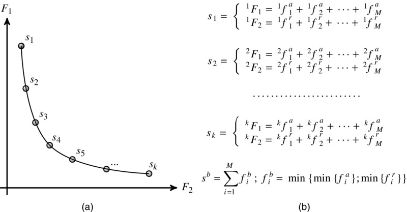
Figure 7.5 (a) The Pareto front of non-dominated solutions to the multi-objective problem in Equations (7.7) and (7.8). Illustrated here is a front of k solutions for a network of M genes. (b) Pareto solutions and the corresponding sum squared errors for individual genes (see the text for details). The overall best solution, sb, is obtained by selected the lowest f value for each gene in turn yielding, in general, a network of mixed regulation types.
To select the best solution, we search the Pareto front to obtain the best parameter values for each connection. As defined in Equations (7.7) and (7.8), the two objectives are determined though the sum of the SSE for each gene in the network. Thus, by retaining the individual gene SSEs, we are able to search the Pareto front to obtain the solution (parameter set) that corresponds to the lowest SSE for each gene. Each solution on the Pareto front has two objective values, each of which corresponds to summed sequence of individual gene SSEs (produced from a specific parameter set), Equations (7.7) and (7.8). Once the optimization process has finished, for each gene, the Pareto front is searched for the parameter set that yields to best objective. Figure 7.5(a) illustrates the Pareto front and Figure 7.5(b) details how each solution corresponds to a summation of individual SSEs for each connection. For each gene, in turn, the front is searched to obtain the solution corresponding to the minimum SSE from either F1 (activating connection, fai) or F2 (repressive connection, fri). That is for each gene we evaluate fai < fri and select the minimum fi that indirectly determines the regulation type. The result is a network containing mixed regulation types that are each selected based on the lowest SSE.
This method has the potential to conduct a better search of the parameter space through its representation as a multi-objective problem. The overhead of searching the Pareto front, performed after the optimization, even for a large number of individuals and genes, is negligible compared to the optimization time. This multi-objective optimization process removes the need for the direct optimization of the regulation type and, therefore, reduces the number of parameters in the problem. Reducing the number of parameters from five to four for each of the n connections results in a large reduction in the search space and could therefore enhance convergence to the global optimum. Here we use 100 individuals and 1000 generations in the optimization stage.
7.4.3 Decoupled Approach
Biological systems are known to be sparse [30] therefore we assume that the connections within the network are independent and treat them as separate, a process known as decoupling [87, 88]. This reduces the dimensionality of the single objective optimization problem from one 5n problem, where n is the number of connections, to n problems each with a dimension of five in the SOS. Here the number five corresponds to the four network parameters and the one Boolean regulation type parameter. Similarly for the MOS, a 4n problem becomes n lots of four dimension problems. Furthermore, due to the decoupling, this technique can also benefit from the use of parallel computation, where each connection can be optimized on a separate CPU. This process can significantly reducing the computational runtime for large networks, though is not implemented here. The objective function here remains the same as for the full network optimization case with the exception of the summation over the number of genes. In this setup Equation (7.6) becomes

Here the total network SSE, ![]() , is calculated after the optimization process is completed by summing the individual connections’ objective value from Equation (7.9),
, is calculated after the optimization process is completed by summing the individual connections’ objective value from Equation (7.9),

for all connections.
In this single objective case xi(t) is based on one of the equations in Equation (7.4) depending on the connection parameter determined by the optimizer as in the full network case. For the multi-objective optimization setup, however, the decoupled method differs slightly. In the multi-objective decoupled arrangement, each connection is optimized in a similar way to the full network case:


However, the selection of solution from the Pareto front is much simpler. In this method, we have a Pareto front for each connection due to the problem being decoupled. Therefore, as we have a minimization problem, the lowest objective value for each connection is always one of the extreme solutions. This is clearly illustrated in Figure 7.6. For each connection we simply evaluate fai < fri to obtain the optimal parameter set and regulation type, see Figure 7.6. Here we use 100 individuals and 100 generations as this setup converges much faster than the full network setup thus requiring fewer generations in the optimization.
![fi
a versus fi
r graph has descending curve with end points s1, s2. Horizontal dotted line from s1 to min[fi
a] on fi
a axis. Vertical dotted line from s2 to min[fi
r] on fi
r axis.](http://images-20200215.ebookreading.net/13/1/1/9781118911518/9781118911518__evolutionary-computation-in__9781118911518__images__ec07f006.jpg)
Figure 7.6 Pareto front of non-dominated solutions to the multi-objective problem, Equations (7.11) and (7.12), with a decoupled arrangement. Solution s1 corresponds to the best activating connection, and s2 corresponds to the best repressive solution, thus evaluating the minimum of these two yields the optimal parameters for each connection.
7.5 RESULTS
7.5.1 Comparing Objectives from Un-Normalized Data
For the case of the un-normalized (raw) data, each of the gene expression profiles within a single network potentially lies on a different scale; thus, determining a network error is not so straightforward. Comparing the SSE between two genes within the same network may be meaningless if the expression profiles vary in scale, with larger scale expression values tending to have larger SSEs. Therefore, if we take the ratio of SSE (δx) and the area of the expression profile (![]() ) for each gene, we are left with a dimensionless quantity, δx′i, that has removed the difference in expression scale:
) for each gene, we are left with a dimensionless quantity, δx′i, that has removed the difference in expression scale:

For each gene, the dimensionless SSEs (δx′i) can be summed to give the total error for the network, ΔX:

where i is the ith network gene and M is the total number of genes within the network. This normalization of the objective functions not only provides a meaningful network error measurement, but it also enables comparison between the different networks and arrangements. We can now compare the raw data setup with the normalized data arrangement directly. No further processing is required for the normalized data case, as each expression profile has the same area; see Equation (7.1). Therefore, Equation (7.13) reduces to δx′i = δxi and the total network error would remain the sum of the errors in the individual genes.
7.5.2 Full Network Optimization
Figure 7.7 shows the box plots of the total network SSE for 50 randomly initialized optimizations of each of the networks. All raw data here are post-processed using Equation (7.14), thus enabling a direct comparison between raw and normalized setup performances.

Figure 7.7 Box plots for the sub-networks for the single and multi-objective setups for both normalized and un-normalized (raw) gene expression data. Box plots are the distribution of sum squared error over 50 independent simulations of each setup. Labels on the x-axis give the sub-network name and the number of target genes within the network. Outliers are given as circles and averages are median values. The dashed line indicates when the problem becomes underdetermined, that is, when the number of genes exceeds the number of data points. SO, single objective; MO, multi-objective.
Raw versus Normalized Data
For the SOS, the use of normalized data yields much lower network errors compared with the raw data. The difference is two orders of magnitude across the entire range of network sizes. This illustrates the benefits of using normalized data as it has produced much better objective values. The SOS normalized distributions are bigger compared to the raw SOS cases for the larger networks; however, the difference between the distributions is still large. For the MOS, the same outcome is seen as for the SOS case. In addition, it also reduces the distribution range for the smaller sub-networks. Figure 7.7 clearly shows that the use of normalized data is beneficial and improves both the SOS and the MOS.
Single versus Multiple Objective Setup
For the raw data, the MOS case produces a large spread of network errors over the 50 simulations indicated by the long box plots, which overlap with the SOS distributions for the three smallest sub-networks. The MOS performs worse than SOS over the whole range of network sizes and appears to diverge with increasing network size. Similar behavior is seen when using the normalized data and comparing the SOS and MOS cases. Both the raw and normalized data SOS results appear to be approximately constant with increase network size, whereas both the MOS experiments increase with network size. The MOS normalized case, however, does not exhibit the larger distributions of network errors as in the SOS case.
The results here indicate that the use of normalized data can improve performance on modeling gene expression for large-scale networks compared to raw data. This improvement is due to the localization of the search space for all genes. Localization enhances convergence of the optimizer and results in lower errors in each gene and, therefore, the whole network. These results also show that an SOS is better than an MOS for both raw and normalized data over the network sizes tested. The MOS with normalized data does outperform the SOS raw arrangement; however, trends indicate that the SOS raw arrangement would perform better than the MOS normalized case for larger networks that tested here. The normalized data set with the SOS performs the best of all the methods tested. Despite the increase in distribution of errors with increasing network size, the trend indicates that increasing network size results in a small increase in the average network error.
7.5.3 Decoupled Network Optimization
Figure 7.8 shows the results from the decoupled approach for the sub-networks modeled. The use of the decoupled methodology leads to much narrower distributions compared to the full network arrangement for both raw and normalized data sets and for both SOS and MOS. In the full network case, some distributions span an order of magnitude, where the largest ones in the decoupled approach are approximately half an order of magnitude, and are the minority. Almost all distributions are so narrow that they are not fully observable in Figure 7.8.

Figure 7.8 Box plots of sum squared error distributions over 50 simulations for the decoupled arrangement, plots as shown in Figure 7.7. A significant difference between the normalized and raw data is clear here with a separation between distributions of around 2.5 orders of magnitude. SO, single objective; MO; multi-objective.
Raw versus Normalized Data
A significant difference between using raw and normalized data is evident in Figure 7.8 where distributions based on data sets are separated by approximately 2.5 orders of magnitude. The use of normalized data has led to a reduction in network error as in the full optimization case. Additionally, the large difference between the RedD network and the other sub-network has greatly been reduced, though it has also led to a slightly wider distribution (taking the scale into account) over the 50 simulations. Also for the SOS, the normalized data have also produced a wider distribution of the PyrR network (relative to the other sub-networks) compared to the raw data. However this distributions is still around 2 orders of magnitude lower than the raw data case.
Single versus Multiple Objective Setup
For the raw data set, the difference between the SOS and MOS is small. For clarity, the distributions shown in Figure 7.8 have been plotted in difference scale in Figures 7.9(a) and 7.9(b) for the raw and normalized data, respectively. The largest ones for sub-networks show that the MOS results in lower total network errors than the SOS, though this difference is small; see Figure 7.9(a). Over the range of sub-network sizes, the decoupled method has removed the poor performance of the MOS and, thus, has led to comparable results to the SOS. For the normalized data, we can see that the MOS produces narrower distributions than the SOS with lower average values in all sub-networks. Moreover, the average value of the MOS distributions is lower than the minimum SOS distribution value for all sub-networks except for RedD. This indicates significant differences between these methodologies, and even in the exception RedD, the median of MOS is below the lower quartile of the SOS. Furthermore, the maximum (excluding outliers) of the MOS is approximately equal to the average of the SOS. This is shown in Figure 7.9(b). From this figure it is clear the MOS with normalized data produces the best performance as it results in the lowest total network error. Moreover, for the four largest sub-networks, the MOS produces narrower distributions that are approximately 15% lower in total network error. This appears to be a stable trend and may indicate that the MOS produces lower network errors for larger sub-networks than SOS in general.

Figure 7.9 Box plots from Figure 7.8 separated for clarity: the performance of both the single objective setup and multi-objective setup (a) on the raw gene expression data and (b) on the normalized gene expression data. SO, single objective; MO; multi-objective.
7.6 DISCUSSION
Using benchmark synthetic data sets is useful in comparing an algorithm’s performance [40, 43, 53]; however, it may not be a true representation of the algorithm’s performance on real data sets. Currently, there are very few studies that use real data and models are not often based on time-series data. Topological models are useful in identifying motifs and functionalities of networks as well as comparing similarities between different networks and organisms. However, dynamic models are vital in our understanding of gene regulation and interactions within a network. Here, we have investigated several techniques and setups for modeling dynamic GRN interactions based on gene expression data. We have investigated the effect of an MOS and observe a performance hindrance when compared to an SOS for a full network optimization technique. This hindrance has less effect when using normalized data, but is still present. When using a decoupled optimization technique, the MOS is a form of multiobjectivization and is comparable in performance to the SOS when using raw data, and performs significantly better when using normalized data. These results show that the use of multiobjectivization can enhance the optimization search through objective decomposition, whereas a multi-objective representation (that is not a form of multiobjectivization) may hinder performance.
We have demonstrated that the use of normalized data leads to reductions in network error compared with raw gene expression data. This reduction is seen in all arrangements, after correcting for gene expression scale to compare setups and network sizes. The improvement through the use of normalized data is due to the localization of the objective search space. By having a universal parameter range, due to all expression profiles being on the same scale, the optimizer can search the objective space much more efficiently than for the raw data case. For the normalized data setup, the optimal solutions for all connections in a network lie within a local region of the parameter space, whereas this is not the case when using raw data. Moreover, the parameter space when using raw data may be vast with optimal connection values far apart for different genes within a network due to expression scale. The normalization of the gene expression data is a straightforward task that can be applied to data sets prior to optimization and has a significant effect on the results as indicated here.
It is clear that in the full network cases the MOS is not providing optimal solutions to the problem. This is a consequence of the methodology, as solutions on the front represent a collection of individual gene SSEs, which are searched to provide the parameter values for each connection. The selection during the optimization is based on the lowest total SSE for a network, that is, the sum of the individual connection SSEs, yielding solutions with low SSE for all connections rather than for individuals. As a result, the optimal parameter values for each connection are not necessarily selected as the overall network SSE may be high. Although, in principle, this sounds analogous to the SOS, the difference lies in the selection during optimization, where solutions are evaluated based on their total SSE and then post-optimization individual connection parameters are selected. This problem of sub-optimality increases with sub-network size leading to a higher rate of increase in SSEs for larger networks in the MOS compared to the SOS.
The performance enhancement using the decoupled case is due to the reduction in the parameter search space. This method improved performance in terms of lower network error and reduced variance between simulations compared to the full network case. The reduced variance is evident by the narrowing of the distributions over the 50 simulations as shown in Figure 7.8 compared to that shown in Figure 7.7. Additionally, we observe a reduction in the number of outliers (simulation results greater/less than 1.5 × median) over the 50 simulations. This is a result of the reduced variance of the distribution and can be attributed to the increased convergence power of the decoupled arrangement to optimal solutions. For the raw data, the SOS and MOS perform comparably over the range of network sizes; however, for the normalized data we observe a clear improvement of the MOS over the SOS. The best combination of objective setup and data type observed here is the MOS decoupled arrangement with normalized data. This produces the lowest network errors for all of the sub-networks investigated here and demonstrated high reproducibility of the results through low variance. Moreover, this methodology is significantly better than the next best combination, SOS decoupled configuration with normalized data, over all network size.
For the largest network used here (332 genes) the computational runtimes for the full network optimization are approximately 20 and 30 min for the SOS and MOS, respectively (for both the raw and normalized data). For the decoupled arrangements, the SOS runtime was approximately 15 min (for both raw and normalized data) and for the MOS, simulations took 20 and 10 min for the raw and normalized data, respectively. Therefore, the MOS method with normalized data has the shortest runtime in addition to providing the best solutions to the problem.
In this work, we have only considered networks where genes are regulated by only one gene. In general, genes may be targeted by more than one regulator that will add an additional layer of complexity to the problem by increasing the search space. However, we have shown here that this simplification can be effective for reconstructing large networks (up to 332 genes) from time-series data. As biological networks are known to be sparse [30], this is a good first approximation and may be sufficient for the majority of networks. Large networks, such as those used here, are likely to contain genes that have additional regulators, thus an extension of this method could be to add additional regulatory connections for genes that the initial method is unable to fit. This can easily be implemented after the method used here and applied to genes where the SSE between the model and data expression profiles is above a threshold. Extending the method this way would only increase the problem complexity when necessary and avoid overfitting by maintaining biological sparsity.
7.7 CONCLUSIONS
The results here suggest that normalized data enhance convergence of this optimization problem and result in consistent solutions, that is, small variance, being obtained over numerous runs. This effect is independent of objective methodology and observed in SOS and MOS for both the full and decoupled optimization arrangements. Furthermore, the use of a decoupled approach also improves consistency between optimization runs; thus, the results of each simulation can be taken with a high degree of confidence as the variance is low in the majority of cases. Additionally, we observe a reduction in outlier solutions when using normalized data. We examine all comparable methods for optimization and conclude that the best performance is obtained by using a decoupled approach with normalized expression data in conjunction with the novel multi-objective technique developed here. This configuration performs better than the single objective alternative for all network sizes, and exhibits a significant reduction in network SSE compared to the full network optimization setup. In Ref. [53], the authors noted that the application for multiobjectivization to larger networks still requires investigation. Here we have demonstrated the effectiveness of such an approach to enhance optimization across various networks that appears independent of increasing network sizes.
We have developed a novel MOS for modeling the dynamic behavior of genes in a given network and demonstrated that a decoupled arrangement multi-objective can outperform a standard single objective approach. Our novel configuration of a decoupled multi-objective optimizer setup performs comparably to a single objective case when using raw gene expression data; however, when using normalized gene expression data, it consistently performs better with increasing network size. The improved performance with increasing network size occurs from a slight reduction in dimensionality for each connection, reduced from five to four variables. Here, the small improvements over each connection lead to greater performance over larger networks. This novel setup shows little dependence on increasing network size and thus can be applied to large-scale network reconstruction problems. In addition, this methodology, in general, exhibits little variation over numerous independent simulations and thus provides consistently good solutions to this problem. Our method is able to escape local optima as, due to the representation of the problem, these solutions are dominated during the optimizations stage, see Section 7.4.2, resulting in narrow distributions of optimized solutions over a number of runs. Furthermore, this multi-objective approach has the smallest computational runtime of the methodologies tested here and can be applied to other networks and data sets.
REFERENCES
- Mustafa Khammash. Reverse engineering: the architecture of biological networks. BioTechniques, 44(3):323–329, 2008.
- Haiyuan Yu and Mark Gerstein. Genomic analysis of the hierarchical structure of regulatory networks. Proceedings of the National Academy of Sciences of the United States of America, 103(40):14724–14731, 2006.
- Patrizia F. Stifanelli, Teresa M. Creanza, Roberto Anglani, Vania C. Liuzzi, Sayan Mukherjee, Francesco P. Schena, and Nicola Ancona. A comparative study of covariance selection models for the inference of gene regulatory networks. Journal of Biomedical Informatics, 46(5):894–904, 2013.
- Guy Karlebach and Ron Shamir. Modelling and analysis of gene regulatory networks. Nature Reviews. Molecular Cell Biology, 9(10):770–780, 2008.
- Takeshi Hase, Samik Ghosh, Ryota Yamanaka, and Hiroaki Kitano. Harnessing diversity towards the reconstructing of large scale gene regulatory networks. PLoS Computational Biology, 9(11):e1003361, 2013.
- Hana El-Samad, Stephen Prajna, Antonis Papachristodoulou, John Doyle, and Mustafa Khammash. Advanced methods and algorithms for biological networks analysis. Proceedings of the IEEE, 94(4):832–853, 2006.
- Mark Schena, Dari Shalon, Ronald W. Davis, and Patrick O. Brown. Quantitative monitoring of gene expression patterns with a complementary DNA microarray. Science, 270(5235):467–470, 1995.
- Eberhard O. Voit and Tomas Radivoyevitch. Biochemical systems analysis of genome-wide expression data. Bioinformatics, 16(11):1023–1037, 2000.
- Oksana Lukjancenko, Trudy M. Wassenaar, and David W. Ussery. Comparison of 61 sequenced Escherichia coli genomes. Microbial Ecology, 60(4):708–720, 2010.
- Giselda Bucca, Emma Laing, Vassilis Mersinias, Nicholas Allenby, Douglas Hurd, Jolyon Holdstock, Volker Brenner, Marcus Harrison, and Colin Smith. Development and application of versatile high density microarrays for genome-wide analysis of Streptomyces coelicolor: characterization of the HspR regulon. Genome Biology, 10(1):R5, 2009.
- Stephen D. Bentley, Keith F. Chater, Ana-M. Cerdeo-Trraga, Greg L. Challis, Nicholas R. Thompson, Keith D. James, David E. Harris, Michael A. Quail, Helen M. Kieser, David Harper, Alex Bateman, Stephanie Brown, Govind Chandra, Carton W. Chen, Mark Collins, Ann Cronin, Andrew Fraser, Arlette Goble, Juan Hidalgo, Tony Hornsby, Simon Howarth, Hsuan-Chung Huang, Tobias Kieser, Natasha L. Larke, Lee Murphy, Karen Oliver, Susan O’Neil, Ester Rabbinowitsch, Marie-Adéle Rajandream, Kim Rutherford, Simon Rutter, Kath Seeger, David Saunders, Sarah Sharp, Robert Squares, Steven Squares, Kate Taylor, Tim Warren, Andreas Wietzorrek, John Woodward, Bart G. Barrell, Julian Parkhill, and David A. Hopwood. Complete genome sequence of the model actinomycete Streptomyces coelicolor a3(2). Nature, 417(6885):141–147, 2002.
- Thomas Schlitt and Alvis Brazma. Current approaches to gene regulatory network modelling. BMC Bioinformatics, 8(Suppl 6):S9, 2007.
- Spencer Angus Thomas and Yaochu Jin. Single and multi-objective in silico evolution of tunable genetic oscillators. In: Robin C. Purshouse, Peter J. Fleming, Carlos M. Fonseca, Salvatore Greco, and Jane Shaw (eds.). Evolutionary Multi-Criterion Optimization, Volume 7811, Lecture Notes in Computer Science, pp. 696–709. Springer, Berlin, 2013.
- Jesse Stricker, Scott Cookson, Matthew R. Bennett, William H. Mather, Lev S. Tsimring, and Jeff Hasty. A fast, robust and tunable synthetic gene oscillator. Nature, 456(7221):516–519, 2008.
- Spencer A. Thomas and Yaochu Jin. Combining genetic oscillators and switches using evolutionary algorithms. In: Yaochu Jin (ed.). Computational Intelligence in Bioinformatics and Computational Biology (CIBCB), 2012 IEEE Symposium on, pp. 28–34, IEEE, New York, 2012.
- David Angeli, James E. Ferrell, and Eduardo D. Sontag. Detection of multistability, bifurcations, and hysteresis in a large class of biological positive-feedback systems. Proceedings of the National Academy of Sciences of the United States of America, 101(7):1822–1827, 2004.
- Chunguang Li, Luonan Chen, and Kazuyuki Aihara. A systems biology perspective on signal processing in genetic network motifs [life sciences]. IEEE Signal Processing Magazine, 24(2):136–147, 2007.
- Didier Gonze. Coupling oscillations and switches in genetic networks. Biosystems, 99(1):60–69, 2010.
- Spencer A. Thomas and Yaochu Jin. Evolving connectivity between genetic oscillators and switches using evolutionary algorithms. Journal of Bioinformatics and Computational Biology, 11(3):1341001-1–1341001-15, 2013.
- Uri Alon. Network motifs: theory and experimental approaches. Nature Reviews Genetics, 8(6):450–461, 2007.
- Uri Alon. An Introduction to Systems Biology: Design Principles of Biological Circuits. CRC Press, Taylor and Francis Group, Boca Raton, FL, 2006.
- Yaochu Jin and Bernhard Sendhoff. Evolving in silico bistable and oscillatory dynamics for gene regulatory network motifs. In: Jun Wang (ed.). Evolutionary Computation, 2008. CEC 2008 (IEEE World Congress on Computational Intelligence). IEEE Congress on, pp. 386–391, IEEE, New York, 2008.
- Ricard V. Solé and Sergi Valverde. Are network motifs the spandrels of cellular complexity? Trends in Ecology and Evolution, 21(8):419–422, 2006.
- Ron Milo, Shai Shen-Orr, Shalev Itzkovitz, Nadav Kashtan, Dmitri B. Chklovskii, and Uri Alon. Network motifs: simple building blocks of complex networks. Science, 298(5594):824–827, 2002.
- Martin Swain, Thomas Hunniford, Johannes Mandel, Niall Palfreyman, and Werner Dubizky. Modeling gene-regulatory networks using evolutionary algorithms and distributed computing. In: Tony Hey, David W. Walker, and Carl Kesselman (eds.). Cluster Computing and the Grid, 2005. CCGrid 2005, IEEE International Symposium on, Volume 1, pp. 512–519, IEEE, New York, 2005.
- Jennifer Hallinan. Gene networks and evolutionary computation. In: Gary B. Fogel, David W. Corne, and Yi Pan (eds.). Computational Intelligence in Bioinformatics, pp. 67–96. John Wiley & Sons, Inc., Hoboken, NJ, USA, 2007.
- George von Dassow, Eli Meir, Edwin M. Munro, and Garrett M. Odell. The segment polarity network is a robust developmental module. Nature, 406:188–192, 2000.
- Dion J. Whitehead, Andre Skusa, and Paul J. Kennedy. Evaluating an evolutionary approach for reconstructing gene regulatory networks. In: Jordan Pollack, Mark Bedau, Phil Husbands, Takashi Ikegami, and Richard A. Watson (eds.). Ninth International Conference on the Simulation and Synthesis of Living Systems (ALIFE9). MIT Press, Cambridge, MA, 2004.
- Piers J. Ingram, Michael P. H. Stumpf, and Jaroslav Stark. Network motifs: structure does not determine function. BMC Genomics, 7:108, 2006.
- Robert D. Leclerc. Survival of the sparsest: robust gene networks are parsimonious. Molecular Systems Biology, 4(213):1–6, 2008.
- Hailong Zhu, R. Shyama Prasad Rao, Tao Zeng, and Luonan Chen. Reconstructing dynamic gene regulatory networks from sample-based transcriptional data. Nucleic Acids Research, 40(21):10657–10667, 2012.
- Irene M. Ong, Jeremy D. Glasner, and David Page. Modelling regulatory pathways in E. coli from time series expression profiles. Bioinformatics, 18(Suppl 1):S241–S248, 2002.
- David Simcha, Laurent Younes, Martin Aryee, and Donald Geman. Identification of direction in gene networks from expression and methylation. BMC Systems Biology, 7:118, 2013.
- Wei-Po Lee and Yu-Ting Hsiao. Inferring gene regulatory networks by incremental evolution and network decomposition. In: Haiban Duan (ed.). Optimization and Systems Biology, Volume 9, Lecture Notes in Operations Research, pp. 311–324, IEEE, New York, 2008.
- Anton Crombach and Paulien Hogeweg. Evolution of evolvability in gene regulatory networks. PLoS Computational Biology, 4(7):e1000112, 2008.
- Hendrik Hache, Hans Lehrach, and Ralf Herwig. Reverse engineering of gene regulatory networks: a comparative study. EURASIP Journal on Bioinformatics and Systems Biology, 8:1–12, 2009.
- Hidde de Jong. Modeling and simulation of genetic regulatory systems: a literature review. Journal of Computational Biology, 9(1):67–103, 2002.
- Alina Sîrbu, Heather J. Ruskin, and Martin Crane. Stages of gene regulatory network inference: the evolutionary algorithm role. In: Eisuke Kita (ed.). Evolutionary Algorithms. InTech, Rijeka, Croatia, 2011.
- Michael Hecker, Sandro Lambeck, Susanne Toepfer, Eugene van Someren, and Reinhard Guthke. Gene regulatory network inference: data integration in dynamic models—a review. Biosystems, 96(1):86–103, 2009.
- Mukesh Bansal, Vincenzo Belcastro, Alberto Ambesi-Impiombato, and Diego di Bernardo. How to infer gene networks from expression profiles. Molecular Systems Biology, 3(78):1–10, 2007.
- Mariana Recamonde Mendoza and Ana Lúcia C. Bazzan. Evolving random Boolean networks with genetic algorithms for regulatory networks. In: Natalio Krasnogor (ed.). Proceedings of the 13th Annual Conference on Genetic and Evolutionary Computation, GECCO’11, pp. 291–298, ACM, New York, 2011.
- Chien-Hua Peng, Yi-Zhi Jiang, An-Shun Tai, Chun-Bin Liu, Shih-Chi Peng, Chun-Ta Liao, Tzu-Chen Yen, and Wen-Ping Hsieh. Causal inference of gene regulation with subnetwork assembly from genetical genomics data. Nucleic Acids Research, 42(5):2803–2819, 2013.
- Christopher A. Penfold and David L. Wild. How to infer gene networks from expression profiles, revisited. Interface Focus, 1(6):857–870, 2011.
- Edward Keedwell and Ajit Narayanan. Discovering gene networks with a neural-genetic hybrid. IEEE/ACM Transactions on Computational Biology and Bioinformatics, 2(3):231–242, 2005.
- Alina Sîrbu, Heather J. Ruskin, and Martin Crane. Integrating heterogeneous gene expression data for gene regulatory network modelling. Theory in Biosciences, 131(2):95–102, 2012.
- Briti Sundar Mondal, Arup Kumar Sarkar, Md. Mahmudul Hasan, and Nasimul Noman. Reconstruction of gene regulatory networks using differential evolution. In: A. M. Shadullah (ed.). Computer and Information Technology (ICCIT), 2010 13th International Conference on, pp. 440–445, IEEE, New York, 2010.
- Andrea Rau, Florence Jaffrzic, Jean-Louis Foulley, and Rebecca W. Doerge. Reverse engineering gene regulatory networks using approximate Bayesian computation. Statistics and Computing, 22(6):1257–1271, 2012.
- Leon Palafox, Nasimul Noman, and Hitoshi Iba. Reverse engineering of gene regulatory networks using dissipative particle swarm optimization. IEEE Transactions on Evolutionary Computation, 17(4):577–587, 2013.
- Michael Weber, Sebastian Henkel, Sebastian Vlaic, Reinhard Guthke, Everardus van Zoelen, and Dominik Driesch. Inference of dynamical gene-regulatory networks based on time-resolved multi-stimuli multi-experiment data applying netgenerator v2.0. BMC Systems Biology, 7:1, 2013.
- Neal S. Holter, Amos Maritan, Marek Cieplak, Nina V. Fedoroff, and Jayanth R. Banavar. Dynamic modeling of gene expression data. Proceedings of the National Academy of Sciences of the United States of America, 98(4):1693–1698, 2001.
- Shinichi Kikuchi, Daisuke Tominaga, Masanori Arita, Katsutoshi Takahashi, and Masaru Tomita. Dynamic modeling of genetic networks using genetic algorithm and S-system. Bioinformatics, 19(5):643–650, 2003.
- Timothy S. Gardner, Diego di Bernardo, David Lorenz, and James J. Collins. Inferring genetic networks and identifying compound mode of action via expression profiling. Science, 301(5629):102–105, 2003.
- Alina Sirbu, Heather J. Ruskin, and Martin Crane. Comparison of evolutionary algorithms in gene regulatory network model inference. BMC Bioinformatics, 11:59, 2010.
- Wei-Po Lee, Yu-Ting Hsiao, and Wei-Che Hwang. Designing a parallel evolutionary algorithm for inferring gene networks on the cloud computing environment. BMC Systems Biology, 8:5, 2014.
- Kay Nieselt, Florian Battke, Alexander Herbig, Per Bruheim, Alexander Wentzel, Øyvind M Jakobsen, Håvard Sletta, Mohammad T. Alam, Maria E. Merlo, Jonathan Moore, Walid A. M. Omara, Edward R. Morrissey, Miguel A. Juarez-Hermosillo, Antonio Rodrguez-Garca, Merle Nentwich, Louise Thomas, Mudassar Iqbal, Roxane Legaie, William H. Gaze, Gregory L. Challis, Ritsert C. Jansen, Lubbert Dijkhuizen, David A. Rand, David L. Wild, Michael Bonin, Jens Reuther, Wolfgang Wohlleben, Margaret C. M. Smith, Nigel J. Burroughs, Juan F. Martn, David A. Hodgson, Eriko Takano, Rainer Breitling, Trond E. Ellingsen, and Elizabeth M. H. Wellington. The dynamic architecture of the metabolic switch in Streptomyces coelicolor. BMC Genomics, 11:10, 2010.
- Antonio Rodríguez-García, Alberto Sola-Landa, Kristian Apel, Fernando Santos-Beneit, and Juan F. Martín. Phosphate control over nitrogen metabolism in Streptomyces coelicolor: direct and indirect negative control of glnr, glna, glnii and amtb expression by the response regulator phop. Nucleic Acids Research, 37(10):3230–3242, 2009.
- Fernando Santos-Beneit, Antonio Rodrguez-Garca, Alberto Sola-Landa, and Juan F. Martín. Cross-talk between two global regulators in Streptomyces: Phop and afsr interact in the control of afsS, pstS and phoRP transcription. Molecular Microbiology, 72(1):53–68, 2009.
- Antonio Rodríguez-García, Carlos Barreiro, Fernando Santos-Beneit, Alberto Sola-Landa, and Juan F. Martín. Genome-wide transcriptomic and proteomic analysis of the primary response to phosphate limitation in Streptomyces coelicolor m145 and in a δphoP mutant. Proteomics, 7(14):2410–2429, 2007.
- Andy Hesketh, Chris Hill, Jehan Mokhtar, Gabriela Novotna, Ngat Tran, Mervyn Bibb, and Hee-Jeon Hong. Genome-wide dynamics of a bacterial response to antibiotics that target the cell envelope. BMC Genomics, 12:226, 2011.
- Gilles P. van Wezel and Kenneth J. McDowall. The regulation of the secondary metabolism of Streptomyces: new links and experimental advances. Natural Products Reports, 28(7):1311–1333, 2011.
- Mamoru Komatsu, Takuma Uchiyama, Satoshi mura, David E. Cane, and Haruo Ikeda. Genome-minimized Streptomyces host for the heterologous expression of secondary metabolism. Proceedings of the National Academy of Sciences of the United States of America, 107(6):2646–2651, 2010.
- Tatsuichiro Higashi, Yuko Iwasaki, Yasuo Ohnisi, and Sueharu Horinouchi. A-factor and phosphate depletion signals are transmitted to the grixazone biosynthesis genes via the pathway-specific transcription activator grir. Journal of Bacteriology, 189(9):861–880, 2007.
- Kenneth J. McDowall, Arinthip Thamchaipenet, and Iain S. Hunter. Phosphate control of oxytetracycline production by Streptomyces rimosus is at the level of transcription from promoters overlapped by tandem repeats similar to those of the DNA-binding sites of the OmpR family. Journal of Bacteriology, 181(10):3025–3032, 1999.
- Mohammad T. Alam, Maria E. Merlo, The STREAM Consortium, David A. Hodgson, Elizabeth M.H. Wellington, Eriko Takano, and Rainer Breitling. Metabolic modeling and analysis of the metabolic switch in Streptomyces coelicolor. BMC Genomics, 11:202, 2010.
- Anushree Chatterjee, Laurie Drews, Sarika Mehra, Eriko Takano, Yiannis N. Kaznessis, and Wei-Shou Hu. Convergent transcription in the butyrolactone regulon in Streptomyces coelicolor confers a bistable genetic switch for antibiotic biosynthesis. PLoS One, 6(7):e21974, 2011.
- Nicholas E. E. Allenby, Emma Laing, Giselda Bucca, Andrzej M. Kierzek, and Colin P. Smith. Diverse control of metabolism and other cellular processes in Streptomyces coelicolor by the phoP transcription factor: genome-wide identification of in vivo targets. Nucleic Acids Research, 40(19):9543–9556, 2012.
- Franois Voelker and Stphane Altaba. Nitrogen source governs the patterns of growth and pristinamycin production in streptomyces pristinaespiralis. Microbiology, 147(9):2447–2459, 2001.
- Martin G. Lamarche, Barry L. Wanner, Sébastien Crépin, and Josée Harel. The phosphate regulon and bacterial virulence: a regulatory network connecting phosphate homeostasis and pathogenesis. FEMS Microbiology Reviews, 32(3):461–473, 2008.
- STREAM Consortium. SysMO project 10: STREAM—global metabolic switching in Streptomyces colicolor. Available from: http://www.sysmo.net/index.php?index=62. Last accessed date 11 November, 2015.
- Mitsuo Ogura, Hirotake Yamaguchi, Ken ichi Yoshida, Yasutaro Fujita, and Teruo Tanaka. DNA microarray analysis of Bacillus subtilis degu, coma and phop regulons; an approach to comprehensive analysis of B. subtilis 2-component regulatory systems. Nucleic Acids Research, 29(18):3804–3813, 2001.
- Yvonne Tiffert, Petra Supra, Reinhild Wurm, Wolfgang Wohlleben, Rolf Wagner, and Jens Reuther. The Streptomyces coelicolor glnr regulon: identification of new glnr targets and evidence for a central role of glnr in nitrogen metabolism in actinomycetes. Molecular Microbiology, 67(4):861–880, 2008.
- Jens Reuther and Wolfgang Wohlleben. Nitrogen metabolism in Streptomyces coelicolor: transcriptional and post-translational regulation. Journal of Molecular Microbiology and Biotechnology, 12(1–2):139–146, 2007.
- Sueharu Horinouchi, Morikazu Kito, Makoto Nishiyama, Kaoru Furuya, Soon-Kwang Hong, Katsuhide Miyake, and Teruhiko Beppu. Primary structure of afsr, a global regulatory protein for secondary metabolite formation in streptomyces coelicolor a3(2). Gene, 95(1):49–56, 1990.
- Sueharu Horinouchi and Teruhiko Beppu. Production in large quantities of actinorhodin and undecylprodigiosin induced by afsB in streptomyces lividans. Agricultural and Biological Chemistry, 48(8):2131–2133, 1984.
- Spencer Angus Thomas and Yaochu Jin. Reconstructing biological gene regulatory networks: where optimization meets big data. Evolutionary Intelligence, 7(1):29–47, 2014.
- Juliane Schäfer and Korbinian Strimmer. An empirical Bayes approach to inferring large-scale gene association networks. Bioinformatics, 21(6):754–764, 2005.
- Matthieu Vignes, Jimmy Vandel, David Allouche, Nidal Ramadan-Alban, Christine Cierco-Ayrolles, Thomas Schiex, Brigitte Mangin, and Simon de Givry. Gene regulatory network reconstruction using Bayesian networks, the dantzig selector, the lasso and their meta-analysis. PLoS One, 6(12):e29165, 2011.
- Marlene Castro-Melchor, Salim Charaniya, George Karypis, Eriko Takano, and Wei-Shou Hu. Genome-wide inference of regulatory networks in Streptomyces coelicolor. BMC Genomics, 11:578, 2010.
- Xiujun Zhang, Xing-Ming Zhao, Kun He, Le Lu, Yongwei Cao, Jingdong Liu, Jin-Kao Hao, Zhi-Ping Liu, and Luonan Chen. Inferring gene regulatory networks from gene expression data by path consistency algorithm based on conditional mutual information. Bioinformatics, 28(1):98–104, 2012.
- Adam A. Margolin, Ilya Nemenman, Katia Basso, Chris Wiggins, Gustavo Stolovitzky, Riccardo D. Favera, and Andrea Califano. ARACNE: an algorithm for the reconstruction of gene regulatory networks in a mammalian cellular context. BMC Bioinformatics, 7(Suppl 1):S7, 2006.
- Jesper Tegnèr, M. K. Stephen Yeung, Jeff Hasty, and James J. Collins. Reverse engineering gene networks: integrating genetic perturbations with dynamical modeling. Proceedings of the National Academy of Sciences of the United States of America, 100(10):5944–5949, 2003.
- Florian Geier, Jens Timmer, and Christian Fleck. Reconstructing gene-regulatory networks from time series, knock-out data, and prior knowledge. BMC Systems Biology, 1:11, 2007.
- Mudassar Iqbal, Yvonne Mast, Rafat Amin, David A. Hodgson, The STREAM Consortium, Wolfgang Wohlleben, and Nigel J. Burroughs. Extracting regulator activity profiles by integration of de novo motifs and expression data: characterizing key regulators of nutrient depletion responses in Streptomyces coelicolor. Nucleic Acids Research, 40(12):5227–5239, 2012.
- Guy Karlebach and Ron Shami. Constructing logical models of gene regulatory networks by integrating transcription factor–DNA interactions with expression data: an entropy-based approach. Journal of Computational Biology, 19(1):30–41, 2012.
- Kevin Y. Yip, Roger P. Alexander, Koon-Kiu Yan, and Mark Gerstein. Improved reconstruction of in silico gene regulatory networks by integrating knockout and perturbation data. PLoS One, 5(1):e8121, 2010.
- Christoph Kaleta, Anna Gohler, Stefan Schuster, Knut Jahreis, Reinhard Guthke, and Swetlana Nikolajewa. Integrative inference of gene-regulatory networks in Escherichia coli using information theoretic concepts and sequence analysis. BMC Systems Biology, 4:116, 2010.
- Nasimul Noman and Hitoshi Iba. Inferring gene regulatory networks using differential evolution with local search heuristics. IEEE/ACM Transactions on Computational Biology and Bioinformatics, 4(4):634–647, 2007.
- Eberhard O. Voit and Jonas Almeida. Decoupling dynamical systems for pathway identification from metabolic profiles. Bioinformatics, 20(11):1670–1681, 2004.
- Mei Xiao, Luwen Zhang, Bing He, Jiang Xie, and Wu Zhang. A parallel algorithm of constructing gene regulatory networks. In: Luonan Chen, Xiang-Sun Zhang, Ling-Yun Wu, and Yong Wang (eds.). Optimization and Systems Biology, Volume 11, Lecture Notes in Operations Research, pp. 184–188, World Publishing Corporation, Beijing, 2009.
- Chao Sima, Jianping Hua, and Sungwon Jung. Inference of gene regulatory networks using time-series data: a survey. Current Genomics, 10(6):416–429, 2009.
- Anne McVittie. Ultrastructural studies on sporulation in wild-type and white colony mutants of Streptomyces coelicolor. Journal of General Microbiology, 81(2):291–302, 1974.
- David A. Hopwood, Hansrudolf Wildermuth, and Helen M. Palmer. Mutants of Streptomyces coelicolor defective in sporulation. Journal of General Microbiology, 61(3):397–408, 1970.
- Juan Soliveri, Krystal L. Brown, Mark J. Buttner, and Keith F. Chater. Two promoters for the whib sporulation gene of streptomyces coelicolor a3(2) and their activities in relation to development. Journal of Bacteriology, 174(19):6215–6220, 1992.
- Strepdb, the streptomyces annotation server. Available from: http://strepdb.streptomyces.org.uk/. Last accessed date 11 November, 2015.
- Klas Flardh and Mark J. Buttner. Streptomyces morphogenetics: dissecting differentiation in a filamentous bacterium. Nature Reviews Microbiology, 7(1):36–49, 2009.
- Andrea Franceschini, Damian Szklarczyk, Sune Frankild, Michael Kuhn, Milan Simonovic, Alexander Roth, Jianyi Lin, Pablo Minguez, Peer Bork, Christian von Mering, and Lars J. Jensen. String v9.1: protein–protein interaction networks, with increased coverage and integration. Nucleic Acids Research, 41(D1):D808–D815, 2013.
- Todd Anderson, Paul Brian, Perry Riggle, Renqiu Kong, and Wendy Champness. Genetic suppression analysis of non-antibiotic-producing mutants of the Streptomyces coelicolor absa locus. Microbiology, 145(9):2343–2353, 1999.
- Todd B. Anderson, Paul Brian, and Wendy C. Champness. Genetic and transcriptional analysis of absa, an antibiotic gene cluster-linked two-component system that regulates multiple antibiotics in streptomyces coelicolor. Molecular Microbiology, 39(3):553–566, 2001.
- Shin Ando and Hitoshi Iba. Inference of gene regulatory model by genetic algorithms. In: Jong-Hwan Kim (ed.). Evolutionary Computation, 2001. Proceedings of the 2001 Congress on, Volume 1, pp. 712–719, IEEE, New York, 2001.
- Yong Wang, Xiang-Sun Zhang, and Luonan Chen. Optimization meets systems biology. BMC Systems Biology, 4(Suppl 2):S1, 2010.
- Melanie Mitchell. An Introduction to Genetic Algorithms. MIT Press, Cambridge, MA, 1999.
- Yaochu Jin and Yan Meng. Emergence of robust regulatory motifs from in silico evolution of sustained oscillation. Biosystems, 103(1):38–44, 2011.
- Dominique Chu. Evolving genetic regulatory networks for systems biology. In: Kay Chen Tan and Jian Xin Xu (eds.). Evolutionary Computation, 2007. CEC 2007, IEEE Congress on, pp. 875–882, IEEE, New York, 2007.
- Spencer A. Thomas, Yaochu Jin, Emma Laing, and Colin P. Smith. Reconstructing regulatory networks in streptomyces using evolutionary algorithms. In: Yaochu Jin and Spencer A. Thomas (eds.). Computational Intelligence (UKCI), 2013 13th UK Workshop on, pp. 24–30, IEEE, New York, 2013.
- Kalyanmoy Deb, Amrit Pratap, Sameer Agarwal, and T. Meyarivan. A fast and elitist multiobjective genetic algorithm: NSGA-II. Evolutionary Computation, IEEE Transactions on, 6(2):182–197, 2002.
- Hans J. F. Moen, Nikolai B. Hansen, Harald Hovland, and Jim Tørresen. Many-objective optimization using taxi-cab surface evolutionary algorithm. In: Robin C. Purshouse, Peter J. Fleming, Carlos M. Fonseca, Salvatore Greco, and Jane Shaw (eds.). Evolutionary Multi-Criterion Optimization, Volume 7811, Lecture Notes in Computer Science, pp. 128–142, Springer, Berlin, 2013.
- Kalyanmoy Deb and Ram Bhushan Agrawal. Simulated binary crossover for continuous search space. Complex Systems, 9:115–148, 1995.
- Yaochu Jin, Yan Meng, and Bernhard Sendhoff. Influence of regulation logic on the easiness of evolving sustained oscillation for gene regulatory networks. In: Chrystopher L. Nehaniv (ed.). Artificial Life, 2009. ALife’09, IEEE Symposium on, pp. 61–68, IEEE, New York, 2009.
- Mariana Recamonde Mendoza and Ana Lúcia C. Bazzan. Evolving random Boolean networks with genetic algorithms for regulatory networks reconstruction. In: Natalio Krasnogor (ed.). Proceedings of the 13th Annual Conference on Genetic and Evolutionary Computation, GECCO’11, pp. 291–298, ACM, New York, 2011.
- Sohei Ito, Naoko Izumi, Shigeki Hagihara, and Naoki Yonezaki. Qualitative analysis of gene regulatory networks by satisfiability checking of linear temporal logic. In: Isidore Rigoutsos, Christodoulos A. Floudas, Junhyong Kim, and Harel Weinstein (eds.). Proceedings of the 2010 IEEE International Conference on Bioinformatics and Bioengineering, BIBE’10, pp. 232–237, IEEE, New York, 2010.
- Hidde De Jong and Johannes Geiselmann. Modeling and simulation of genetic regulatory networks by ordinary differential equations. In: Edward R. Dougherty, Ilya Shmulevich, Jie Chen, and Z. Jane Wang (eds.). Genomic Signal Processing and Statistics, Hindawi Publishing Corporation, New York, pp. 201–239, 2005.
- Jie Xiong and Tong Zhou. Gene regulatory network inference from multifactorial perturbation data using both regression and correlation analyses. PLoS One, 7(9):e43819, 2012.
- Tim Hohm and Eckart Zitzler. Multiobjectivization for parameter estimation: a case-study on the segment polarity network of Drosophila. In: Günther Raidl (ed.). GECCO’09: Genetic and Evolutionary Computation Conference (GECCO 2009), pp. 209–216, ACM, New York, 2009.
- Julia Handl, Douglas B. Kell, and Joshua Knowles. Multiobjective optimization in bioinformatics and computational biology. IEEE/ACM Transactions on Computational Biology and Bioinformatics, 4(2):279–292, 2007.
- Kalyanmoy Deb. Multi-Objective Optimisation using Evolutionary Algorithms, 1st ed. Wiley, Kanpur, India, 2001.