
CHAPTER 10
USING EVOLUTIONARY ALGORITHMS TO STUDY THE EVOLUTION OF GENE REGULATORY NETWORKS CONTROLLING BIOLOGICAL DEVELOPMENT
Alexander Spirov
Computer Science and CEWIT, SUNY Stony Brook, Stony Brook, NY, USA; and the
Sechenov Institute of Evolutionary Physiology and Biochemistry, St.-Petersburg, Russia
David Holloway
Mathematics Department, British Columbia Institute of Technology,
Burnaby, B.C., Canada
10.1 INTRODUCTION
Developmental biologists approach the embryological formation of organisms in terms of the temporal and spatial regulation of gene expression. How does gene regulation precisely specify in what cells and at what time a gene is expressed (to a given level)? Much of the work in the field is on the gene–gene interactions, frequently in extended regulatory networks, which control given events in development.
Computational work on developmental gene regulatory networks (GRNs), to construct the “wiring diagrams” of gene connections and characterize network dynamics, has been going for many decades. More recently, there has been increasing focus on the evolutionary dynamics of how these GRNs arose. Since developmental GRNs are fundamental to creating the body plan of a species (and the functions associated with the form), understanding the evolution of GRNs is fundamental to understanding the dynamics of speciation: how is an organism’s form (phenotype) maintained, despite environmental variation and genetic mutation, and how is such stability balanced against evolvability, or the potential to respond with fit phenotypic changes to environmental or genetic changes? Computational simulations of GRN evolution have become very powerful tools for addressing such fundamental issues in evolutionary theory. At the same time, evolutionary algorithms (EAs) have become a major approach for optimization problems. EA has been inspired by the general principles of biological evolution, such as mutation, selection, and reproduction. We feel there is a large potential for developing new EA techniques based on more detailed mechanisms of biological evolution, for instance, using sexual reproduction or retroviral mechanisms of gene crossover. At the same time, the techniques used by computational biologists simulating evolution can be computationally intensive, and could benefit from improvements from computer science EA approaches (e.g., Ref. [1]). For a recent methodological guide to the computational biology of evolutionary simulations, see also Ref. [2].
In general, we will be discussing evolutionary computations with the general cycle (Figure 10.1):
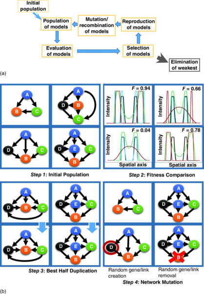
Figure 10.1 Overview of evolutionary computation approach. (a) General cycle of evaluation, selection, reproduction, and mutation to create spatial gene expression patterns (see the text). F-values represent the relative fitness for each spatial pattern. (b) A more detailed schematic of this process, for an initial population of GRNs (Step 1), evaluation for fitness to produce a particular spatial gene expression pattern (Step 2), selection and reproduction of the fittest GRNs (Step 3), and GRN mutation (Step 4), changing parameters (kinetics) or the network connections themselves, as shown here (after Ref. [3]).
- An initial population is chosen. In simple cases, individuals can be different parameter sets for a given GRN; more complex cases include individuals with different connectivities or member genes.
- Individuals are tested for fitness against given criteria. For example, for spatial expression problems, individuals are scored by how well they recreate experimental patterns (e.g., an individual’s parameters are used in a differential equation model of the patterning process, and the simulated pattern is scored against experimental data).
- Low-scoring individuals are selected out of the population.
- New individuals are introduced into the population to replace those just selected out. Generation of new individuals can be specified by inheritance rules from parent individuals.
- Parameters are mutated. This can, for example, alter gene–gene interaction strengths, including adding or eliminating interactions. More detailed approaches can mutate at a gene’s sequence level, for example, altering cis-regulatory sequences (to alter regulator binding strengths), or distinguishing between point mutation and crossover operations, which involve entire regions of a sequence.
- Steps (b)–(e) are repeated for some number of generations.
In this chapter, we will outline the general approaches being used by computational biologists to simulate evolution, and review some of the major impacts this work is having on biological theory (especially, understanding the dynamics of evolution). With this survey of evolutionary simulation, we aim to inspire computer scientist practitioners of EA with the biology, as well as pointing to areas in the biological modeling, which could most benefit from increased computational efficiencies.
10.2 COMPUTATIONAL APPROACHES FOR THE EVOLUTION OF DEVELOPMENTAL GRNS
We distinguish two broad approaches for simulating GRN evolution in developmental problems. The first, the “coarse-grained” approach, treats the genes as nodes and their interactions as edges in a network (as depicted in Figure 10.1). The interactions and their strengths can be coded as a regulatory matrix. This approach has been used very extensively for studying evolutionary principles over the past two decades. It is, however, coarse grained in the sense that real gene regulation and biological evolution both operate at the deoxyribonucleic acid (DNA) sequence level. Fine-grained approaches have been increasingly developed in recent years, modeling at the level of sequence information (or at least a region of sequence, or regulatory module). With the corresponding increase in genome sequencing and comparative genomics, this provides powerful predictive value for evolutionary dynamics at the molecular genetic level.
10.2.1 Coarse-Grained Approaches
Coarse-grained simulations of GRN evolution were pioneered by Andreas Wagner et al. [4, 5]. In their approach, genes are nodes of the network, which interact (network edges) only one on one (co-factors are not modeled), leading to Boolean (on–off) expression levels. These assumptions are too simple for a number of developmental phenomena (such as spatially patterned gene expression in response to a concentration gradient of a regulator), but the models are very fast to solve, and have had significant impact on the understanding of evolutionary principles (see Ref. [6] for further perspective).
10.2.1.1 W Matrix
In Wagner’s core model, a GRN is represented by the state of the network genes 1 − N:
Si(t) is binary—the gene is either expressed or not. Cross- and autoregulatory interactions causing the state to change are modeled by difference equations:

where the expression state of gene Gi at time t + τ, Si(t + τ), is a function of a weighted sum, hi(t), of the expression state of all network genes at time t. σ(x) is the sign function (σ(x) = −1 for x < 0, σ(x) = +1 for x > 0 and σ(0) = 0), and τ is a time constant whose value depends on biochemical parameters such as the rate of transcription or the time necessary to export mRNA into the cytoplasm for translation. The real constants wij represent the strength of regulatory interaction of the product of Gj with Gi, (activation, wij > 0; repression, wij < 0). wij are the elements of the W matrix representing regulation in the GRN. The approach is shown schematically in Figure 10.2; see Ref. [7] for a recent review.

Figure 10.2 Representation of a GRN via the connectivity or regulation matrix W = Wi ← j (the W element represents the action of the jth gene on the ith gene; can also be written as Wij). (a) Matrix representation of gene regulation by transcription factors (TFs) encoded by the genes. In biological terms, the wijs represent both the TF binding strength and the transcriptional activation (or repression) ability of the jth factor on the ith gene. wij values are relative. The ith row of W corresponds to the entire cis-regulatory region of gene Gi. The matrix W = (wij) corresponds to all regulatory DNA elements relevant to regulatory interactions among network genes. The more zero entries W has, the fewer regulatory interactions exist among network genes. (b) Each gene (horizontal arrow) is regulated by the products of the other genes (boxes). Strength and direction of regulation (depicted as different color saturation levels) are a function of both the regulatory element and the abundance of its corresponding gene product. Genotype is represented as the matrix W, and phenotype is the vector TF.
10.2.1.2 Extensions of the W Matrix Approach
The W matrix approach has been used extensively over the past two decades. To address particular topics, it has been refined and extended in a number of ways.
Interaction function
Siegal and Bergman [8, 9] introduced a sigmoidal function for σ in Equation (10.2) that allowed for dynamic switching of a repressive state into an activating state. This was then extended to allow for recombination (allele r or R, with equal probability) to modify σ [10]. Masel [11] set σ(x) = 1 (expressed) if x ⩾ 0 and σ(x) = 0 (not expressed) if x < 0, a more realistic mapping, biologically, than the negative values allowed in Equation (10.2). The balance between activating and inhibiting connections in W matrix models, including oscillations, was explored by McDonald et al. [12].
Co-factors
Biological gene regulation in eukaryotes commonly involves co-factors, in which the effect of a transcription factor (TF) is amplified or diminished by the presence of a different TF. Extension to a triple-index representation, Wijk, allows for TFs j and k to simultaneously affect the expression of gene i [13].
Spatially distributed gene expression
A critical aspect of developmental gene expression is its spatial dependence; genes must be expressed in distinct domains in order for tissues to differentiate in the correct locations. Although simulations of spatially dependent GRNs have a long tradition in developmental biology, it is more recently that the evolution of these GRNs has been studied. Anterior–posterior segmentation of the insect body plan is extremely well characterized through comparative biology, as well as through developmental biology of the fruit fly Drosophila melanogaster, and has become a test case for evolutionary simulations of spatially dependent gene expression. While Boolean gene states have been used with spatial patterning, researchers are generally turning toward continuous (DE) representations of gene states, to address the concentration-dependent aspects of developmental patterning. Evolutionary coarse-grained segmentation models include those of Salazar-Ciudad et al. [130, 131]; Sole et al. [14], Francois et al. [15, 16], Fujimoto et al. [17], and ten Tusscher and Hogeweg [18, 19] (overview of their approach shown in Figure 10.3). For reasons of computational simplicity, these models assume a one-dimensional embryo consisting of a row of cells (Figure 10.3b), ignoring morphogenetic processes and patterning in higher dimensions. Some of these network models, (Refs. [18, 19, 15, 16])are still Boolean and do not incorporate diffusion or transport for modeling spatial pattern formation, while others (Refs. [130, 131, 17]) have developed continuous evolutionary models for insect segmentation, with Hill-equation kinetics. With the exception of the work in Refs. [18, 19], which used a genome encoding the regulatory network, studies used the GRN directly as the genotype, with mutations occurring directly on the network (as depicted in Figure 10.3c) rather than on the genome sequence. The approaches differed, in details, on how the genotype is mapped to the phenotype (Figure 10.3b and Ref. [19]); please see Ref. [19] for a recent review on how these evolutionary developmental simulation studies shed light on some classic biological problems.

Figure 10.3 An example of modeling evolution of a GRN controlling spatially dependent gene expression, in this case anterior–posterior segmentation of the fly body plan. (a) The population of individuals, each with a GRN. (b) GRN topology specifies the gene expression response to a maternal signaling gradient (modeled continuously with DEs). This produces variations on a striped expression pattern. (c) GRNs are mutated. (d) The reproduction chances of individuals are fitness based; fitness increases with the segment number. Reprinted with permission from Ref. [19], copyright 2013 Springer Science and Business Media.
10.2.1.3 Increased Efficiency in Solving Coarse-Grained Models
Though an advantage of coarse-grained approaches is their speed, several groups have worked on improving computational efficiency, in order to access larger numbers of generations (simulation cycles), particularly for spatially dependent models. Fomekong-Nanfack et al. [20] developed an evolutionary strategy (ES) for finding parameters in segmentation models, some 5–140 times faster than an earlier parallel simulated annealing approach [21]. Their “island” ES algorithm operates on N populations of individuals, each with a population size of i. Simulation cycles are generally run within islands, with the best individuals copied between islands every m generations. Jostins and Jaeger [22] developed an asynchronous communication between parallel islands that offered further speed-up. A different parallel method, DEEP (Differential Evolution Entirely Parallel), has been developed by Kozlov and Samsonov [23].
10.2.1.4 Digital Organisms
At a more general level, evolution has been studied within the framework of artificial life. Digital organisms can replicate, mutate, and have fitness criteria. This approach does not tend to address the biological details of gene regulation, but it can offer a platform to study general principles of evolving systems. For instance, Lenski et al. [24] used two classes of organism; one simple (rapidly replicating) and one complex (able to accelerate replication according to “metabolic” rewards). They found, after millions of mutations were introduced, that the complex organisms were more robust to single mutations than the simple organisms. Ofria et al. [25] found that while traits may appear suddenly in an evolutionary process, the information content of the genome is gradually varying. They argued that “… it is nearly impossible for a significantly complex trait to appear without reusing existing information.” Clune et al. [26] addressed the classic question of whether ontogeny recapitulates phylogeny, finding, in digital organisms, that traits that evolved earlier tended to occur earlier in an individual’s development. By adding a type of epistasis (gene background effect), Valverde et al. [27] observed that modular control of expression (clustered gene effects) was spontaneously generated (also see Section 10.2.2.2). Covert et al. [28], using digital organisms, described how deleterious mutations could be beneficial, opening access to new regions of the fitness landscape. Batut et al. [29] applied digital organisms to the evolution of marine cyanobacteria; matching observations that reduced selection strength led to genome loss, with a majority of the loss in non-coding sequences.
10.2.2 Fine-Grained Approaches
To address the biology more realistically, a number of groups have incorporated DNA structure into evolutionary models. The finer level of detail brings significant computing costs, but can answer evolutionary questions on the molecular genetic level (see, e.g., the review in Ref. [30]). Different levels of abstraction can be made within the fine-grained approaches. It is rare to model at base-pair resolution, but a number of groups include TF binding sites (TFBSs; including cooperative or competitive effects between TFs), as well as addressing the modular structure of cis-regulatory regions (reflecting that many genes have multiple enhancers [31, 32]).
10.2.2.1 Evolution of TFBSs
ten Tusscher and Hogeweg [33] extended the basic W matrix approach to allow for multiple TFBSs. This allowed them to model different types of mutations: in TFBSs; in the coding part of the gene; as well as those affecting segments of the genome (see also Ref. [34]). At slightly more detail, Pujato et al. [35] included structural models of TF–DNA complexes to find binding strengths. Mutation altered TFBS strengths and created or destroyed binding sites (BSs). The Sinha group [36, 37] has developed thermodynamic models for binding individual TFBSs and for entire cis-regulatory modules (CRMs). Simulations of TFBS evolution for 37 well-characterized CRMs in Drosophila segmentation corroborated the BS conservation at short times and BS loss at longer times seen across 12 Drosophila genomes.
10.2.2.2 Evolution of Modular Control
Many genes have multiple CRMs, with distinct sequences of TFBSs. For spatial patterning, different CRMs can control different regions of gene expression. We have developed a model for the evolution of multiple CRM structure in one of the major Drosophila segmentation genes, hunchback (hb) [38, 39]. Figure 10.4(a) shows some of the experimentally determined structure, in terms of BSs for specific hb TFs, separated into two of the three known enhancers active during segmentation. Figure 10.4(b) shows how we represent this structure in symbolic strings. The expression levels of hb depend on the arrangement of activating and repressing TFBSs, modeling co-activation and co-repression. In each generation of an evolutionary computation, hb spatial patterns are selected against experimental hb patterns. TFBSs mutate and evolve to optimize fits to the data. We have shown that the multiple CRMs observed in hb could have readily evolved.

Figure 10.4 Representation of hb regulatory region (after Ref. [39]). (a) Schematic of two of the hb cis-regulatory modules (CRMs), showing binding sites (BSs) for specific TFs (visualized with Genamics Expression software). (b) Representation of the BS for hb TFs (Bcd—B, Cad—C, Ems—E, Gt—G, Hb—H, Kr—K, Kni—N, Tll—T, etc.) as strings of characters, neglecting distance along the DNA between BSs. Asterisks denote spacers (non-BS DNA) separating CRMs. (c) Strength of an activating BS is calculated by a three-step algorithm which sums activation (including co-activation) and repression strengths dependent on neighboring TFs (a short action radius of three BSs is used): (1) local activation strength is tallied; (2) neighboring activation is added; (3) neighboring repression is added. The summed action strength is shown at the bottom of the figure.
10.3 USING EVOLUTIONARY COMPUTATIONS TO INVESTIGATE BIOLOGICAL EVOLUTION
Evolutionary computations have been applied in a number of areas, allowing researchers to test the limits of theoretical concepts. This has led to a number of refinements of classic evolutionary theory in recent years.
10.3.1 Evolvability and Robustness
Several related concepts from the 1950s have had a major impact on the evolutionary theory of development. These include canalization, whereby species show low phenotypic variation, despite ample genetic and environmental variation (also termed as “robustness” [40, 41, 42]; and genetic assimilation, in which a phenotypic change induced by an environmental perturbation becomes stabilized in the genotype [43, 44].
10.3.1.1 Canalization
The understanding of how canalization operates has been greatly advanced in recent years through evolutionary modeling (reviewed in Ref. [45]). A number of different computational approaches have exhibited canalization, highlighting different aspects of the evolutionary mechanisms involved.
Stabilizing selection (in which individuals are removed from both ends of a phenotypic distribution, maintaining the mean) has been shown, by modeling at several levels, to contribute to canalization. In simulations where phenotypes had different degrees of sensitivity to microenvironmental variation (developmental noise [46]), stabilizing selection produced canalization. Explicit modeling of individual development and evolution also showed this [4]. Modeling at the population-genetic level, Wagner et al. [47] distinguished that canalization against environmental variation can increase with stabilizing selection, but canalization against mutation increases only up to a point. Above a threshold, stabilizing selection purges the genetic variation from a population, and genetic canalization no longer applies.
Indeed, further work indicates that selection for environmental canalization may produce genetic canalization as a by-product [8, 9], that more densely connected networks evolve to be more robust to perturbation than sparser networks under stabilizing selection, and that phenotypic robustness to genetic perturbation does not directly indicate adaptive canalization (reviewed in Ref. [48]). Siegal and Bergman’s [8] simulations indicate that increased GRN complexity is associated with robustness. Canalization is not due to direct selection for reduced variability, but because GRNs evolve complexity to buffer against the effects of lethal gene deletions. “We argue that canalization may be an inevitable consequence of complex developmental-genetic processes and thus requires no explanation in terms of evolution to suppress phenotypic variation” [8] (see also Refs. [5, 49]). Systematic computational tests of how an arbitrary null (knockout) mutation affects the expression of other genes reveal that arbitrary genes in complex gene networks have the property of buffering genetic variation and, therefore, have the potential to act as evolutionary capacitors. In a complex GRN, there are many gene products which could appear as “phenotypic” capacitors, such that their removal increased phenotypic variability [9]. This is consistent with experimental observations that the buffering of other genes’ expression levels is disrupted when a single gene is knocked out. An extensively studied example is the molecular chaperone Hsp90 [50, 51], but GRN dynamics suggest there should be many more. Experiments in yeast have indicated more than 300 gene products whose removal increased variation [52]. Leclerc [104] has noted that real gene networks appear to be robust, but tend to be sparsely, not densely, connected. He showed that when the costs of complexity are taken into account, that robustness implies a parsimonious network structure that is sparsely connected; that selection will favor sparse networks when topology is free to evolve.
Gombar et al. [53] simulated epigenetic regulation (e.g., chromatin remodeling), and found that this not only facilitated decoupling of mutational and environmental robustness, but it also increased GRN sensitivity to noise (without the loss of robustness). The authors speculated that this epigenetic effect was a necessary condition for multicellularity to arise. Furusawa and Kaneko [54] found that positive feedback through epigenetic regulation aids fast and precise evolutionary responses to environmental change.
Canalization as a by-product of selection against environmental variation appears to be quite general, being seen in simulations of ribonucleic acid (RNA) evolution [55] and metabolic network evolution [56] (where it was suggested that environmental noise is needed for metabolic networks to be robust to gene loss). In general, “It may be that any developmental system that greatly reduces the dimensionality of phenotypes relative to the dimensionality of genotypes will produce the appearance of canalization by releasing hidden genetic variation when perturbed” [48].
10.3.1.2 Genetic Assimilation
As Waddington first stated the genetic assimilation concept, “… if selection was practiced for the readiness of a strain of organisms to respond to an environmental stimulus in a particular manner, genotypes might eventually be produced which would develop into the favoured phenotype even in the absence of the environmental stimulus. A character which had originally been an ‘acquired’ one might be said to have become genetically assimilated” [43] (see also Refs. [40, 44]). Computations in the past decade have refined this idea. For instance, Masel [11], using a variant of the Wagner model (Section 10.2.1.2), showed that genetic assimilation can occur in the absence of selection for the trait.
Genetic assimilation requires an underlying phenotypic plasticity—a capacity for the genotype to produce multiple phenotypes in response to non-genetic perturbations [57, 58, 59]. A factor in this response is the release of cryptic genetic variation, which occurs due to neutral drift, but may be invisible until a large enough perturbation occurs [60]. Mathematical analysis of Wagner’s canalization model [61] indicates that evolution toward a particular phenotype stabilizes other (cryptic) phenotypes, making GRNs more robust to genetic perturbations (loss, mutation, etc.). Computations by Lande [62] quantify the relation between plasticity dynamics and assimilation, wherein plasticity must increase in order to allow evolution to a perturbed environment, but then decrease in order to maintain the new optimum. Espinosa-Soto et al. [63] also characterized the plasticity–assimilation relation, using classic W-matrix simulations [64].
10.3.1.3 Noise
Lehner and Kaneko [65] have used an approach from statistical physics to derive a “fluctuation–response” relation for evolution akin to the “fluctuation–dissipation” theorem relating Brownian noise and motion in fluids. This describes a fundamental relation between environmental noise and evolvability. They found an optimal range of noise, which could contribute to evolution: above a critical noise level “error catastrophe” resulted; below this, GRNs can get stuck in fitness landscapes, and not evolve due to perturbations (i.e., low plasticity) [66, 67, 68]. They also found that evolution of robustness to noise could result in robustness to genetic mutation (similar to Ref. [8]), due to a proportionality between the environmental (noise) and genetic (mutation) contributions to phenotypic variance [69, 70, 71, 72].
A number of these projects used numerical simulations to explore the theoretical principles. In Ref. [67], it was found that networks acquired both mutational and noise robustness if the phenotypic variance induced by mutations was smaller than that observed in an isogenic population (where variance is only due to gene expression noise). They found adaptive states, characterized by high production and decay terms, were also less affected by gene expression noise. Developmental noise could aid both adaptability and robustness, with the highest adaptability at high noise levels that nearly destroy robustness.
In Ref. [71], two interacting and evolving networks were modeled: one a GRN controlling protein expression and the other a metabolic network depending on the GRN proteins and environmentally supplied nutrients. Growth of the “cell” containing these networks is limited by metabolite influx. They found that in any cell with stochastic gene expression, the cell’s state was selected by noise—it did not need to be driven by a specific signalling network.
Kuwahara and Soyer [73] used an intrinsic method (Gillespie algorithm) to model noise in a gene with autofeedback, and corroborated that noise (in the resulting bistable switch) aids evolvability. Extending the approach to consider protein–gene and protein–protein interactions, van Dijk et al. [74] have predicted that GRNs with monomeric TFs, rather than dimeric, are more robust to mutations affecting regulatory interactions.
Quantifying Waddington’s concept, Kaneko [75] identified genetic assimilation as the proportionality between genetic and environmental contributions to phenotypic variability. He found that the number of genes with environmental contribution greater than genetic contribution increased as robustness of fitness increased, with a concomitant decrease in the degrees of freedom for gene mutation [76].
10.3.1.4 Adaptation
Biologically, stable end states might not be the critical feature for speciation or survival. How fast a species approaches a stable state, its rate of adaptation, might be more important. Genes in a GRN will generally change expression in response to an environmental perturbation, with some genes returning rapidly to prior levels and some maintaining altered expression to adapt [77]. Neyfakh et al. [78], using a simple model of a cell with a GRN controlling basic metabolism of an environmental nutrient, found a rapid rise in fitness in response to an environmental perturbation, which then plateaued. The resulting GRNs were quite diverse, many with what appeared to be functionally non-essential genes (see also Section 10.3.3.1 on gene co-option). Cuypers and Hogeweg [79] (reviewed in Ref. [80]) further worked with this model, and found that the plateauing after the initial rise in fitness could be characterized by a period of streamlining gene loss.
Does this dynamic merely reflect the plasticity needed for genetic assimilation, or does plasticity itself affect adaptation rate (i.e., what is the relation between plasticity and evolvability)? Fierst [81], using the Wagner model [4], showed that “a history of phenotypic plasticity may … shorten the waiting time for the generation of phenotypic variance from new mutations and recombination. Rather than acting as a short-term alternative, phenotypic plasticity may facilitate future adaptation and genetic evolution.” On the other hand, plasticity can contribute to liability in developmental GRNs. Draghi and Whitlock [82], with a continuous extension of Wagner’s model [5], quantified how phenotypic plasticity increased variance, in mutations and in standing genomes, which could be amplified for correlated genes.
Francois and Siggia [16] (see also Refs. [83, 84]) used small GRNs to characterize two finer aspects of the response to perturbations: responsiveness, the speed at which genes altered expression, and quality of adaptation, or how well the GRN maintained fitness to the new environmental condition (see also Ref. [85] for an application to temperature compensation in circadian clocks). Ma et al. [86] did a complete analysis of all 3-node GRNs, and found only two topologies with an adaptive response, a negative feedback loop with a buffering node and an incoherent feed-forward loop (FFL). However, this does not appear to generalize to large GRNs: simulations with large GRNs [77] did not find few gene motifs underlying adaptation; rather, adaptation was cooperative across the network (and contributed to robustness).
Modeling has made the original concepts of Waddington much more precise; the quantitative questions raised by the modeling, such as what degree of plasticity is optimal for the development of particular organisms, may now be at the stage to allow for experimental testing.
10.3.2 Crossover
Genetic material is altered in mutation and in reproduction. Both have profound impacts on evolutionary dynamics. There is great potential to refine EA by drawing from the details of biological reproduction mechanisms. In particular, point mutation tends to destroy meaningful “words” (genes) in the process of evolution; crossover of longer segments of genetic material can maintain these building blocks [87, 88]. For instance, Martin and Wagner [7] added recombination and point mutation steps to the W matrix approach and reported that recombination may be a much stronger factor in GRN evolution than point mutation. When both steps are active, they found genotype diversity to be increased, the deleterious effect of point mutations to be decreased, and the emergence of cis-regulatory complexes (combinatorial regulatory interactions). In this section, we discuss several approaches to simulating reproduction mechanisms and how this reflects on the role of reproduction in evolutionary dynamics.
10.3.2.1 Sexual Reproduction
The role of sexual reproduction in evolution has been intensively studied, and has long been understood to increase population fitness. Azevedo et al. [89] quantified this effect using an extension of the W matrix approach (see also Ref. [33] for sexual reproduction in W matrices). At closer detail, Livnat et al. [90, 91] argued that sex does not maximize fitness generally, but specifically improves mixability, the capacity of a particular genome to function with a wide variety of genetic partners. Sex also has the potential to destroy favorable combinations of genes. Misevic et al. [92, 93] used a digital organisms’ approach to compare sexual reproduction and asexual reproduction. They found clustering of genes (modularity) for similar traits with sexual reproduction, which may contribute to maintaining desirable characteristics.
Sexual reproduction frequently involves sexual selection, which can drive sexual dimorphism. Rapid evolution of dimorphism suggests that the underlying GRNs may favor evolvability over phenotypic stability. However, Fierst [81, 94] found, with a W matrix approach, that GRNs could produce dimorphic characteristics with both high robustness and high evolvability; coarse-grained dynamics may have the capacity to do both things.
Heterosis, or “hybrid vigor,” is the tendency for crosses of individuals from genetically distinct populations to improve particular traits (e.g., growth rate). Emmrich et al. [95, 96] have recently developed a GRN evolutionary simulation approach with hybridization to quantify this process.
10.3.2.2 Retroviral Crossover
Sexual reproduction is not the only mechanism used in biology for crossover of large segments of intact genetic information. We have developed a genetic algorithm (RetroGA) with crossover inspired by the mechanism by which retroviruses create DNA strands from RNA [87, 88] (which is then copied into a host). Biologically, the DNA strand is generally produced from two parent RNA strands, with the read-off switching between strands depending on jump sequences (regions of homology). We have tested this mechanism on Royal Road and Royal Staircase functions [97], designed to evaluate the retention of building blocks (e.g., genes), as well as on biological test cases in bacterial promoter evolution and Drosophila segmentation. These tests are characterized by basin-subportal architecture of the fitness landscape, with long periods of neutral evolution followed by quick jumps to higher fitness (upon creation of a new building block). In all cases, the RetroGA algorithm significantly sped up evaluation in comparison to point mutation.
10.3.3 GRN Outgrowth
GRNs can change size in the process of evolution, by gaining or losing genes. Genes can be newly created or destroyed within a GRN. But it is likely much more common for pre-existing genes to have small mutations in their CRMs, which allows them to be regulated by TFs from other GRNs, effectively recruiting them into that GRN [98, 99]. A number of groups have simulated ways in which simpler ancestral GRNs can evolve into more complex derived GRNs.
10.3.3.1 Gene Co-Option
Computations indicate that co-option (recruitment) of genes and outgrowth of GRNs (increase in network nodes) occur spontaneously, without particular selective pressure for network complexity. Incorporating gene addition and gene withdrawal operators into a standard GA, we found a net increase of genes in GRNs (Figure 10.5) [100, 101]. We tested the algorithm on a coarse-grained (continuous, partial DE) GRN model for Drosophila segmentation, and found that the derived networks showed increased developmental robustness to fluctuations in maternal signalling factors. Co-opted genes frequently matched experimentally observed patterns, and became essential nodes of the derived GRN. Similar facility of network outgrowth has been observed in Ref. [102]. In simulations of protein networks, these authors found that adding mechanisms for protein addition, duplication, or deletion, as well as creation or destruction of interactions produced network growth, in the absence of any specific selection pressure for larger networks. Tsuda and Kawata [103] found similar results with a fine-grained GRN model (with TF binding in individual CRMs): complex GRNs tended to evolve if beneficial gene duplications were fixed in the genome. In the very fine-scaled work of He et al. [36], which was corroborated against Drosophila sequence data and expression patterns, it was observed that complex networks were favored by the evolutionary process (characterized by large numbers of TFBSs in the enhancers). With relevance also to Section 10.3.1, Pujato et al. [35] found that in simpler GRNs (with less connections) robustness (to environmental perturbations) depended on local sequences decreasing the creation or destruction of TFBSs. For more complex GRNs (with more connections), robustness depends on regulating TFBSs with high-level network wide effects. Iwasaki et al. [60] found a strong correlation between the amount of cryptic variation and the network size, leading them to propose that network expansion could be a source of evolvability. Work by Leclerc [104] places some caution on universal GRN outgrowth: if a cost is entered for GRN complexity, evolution can favor sparser networks.

Figure 10.5 Modeling co-option of a new gene into a network during evolution. (a) Initial n-gene network (G1, … , Gn), producing n TFs ( , … ,
, … ,  ). (b) New gene (GC1), producing a new factor
  , can be incorporated by chance and retained if it maintains or improves fitness (gray colored row and column). The initial n-gene network can become completely rewired by co-opting GC1.
Computations suggest that gene co-option can provide robustness to a GRN from parasite attack. In studies of co-evolution of a host and a parasite, Salathe and Soyer [105] found that parasite selective pressure led to recruitment and retention of new nodes to a host GRN, which buffered the host to loss of particular genes. When the parasites were removed, the host GRN could shrink again without the loss of fitness.
In several studies [106, 107, 108], we have characterized how gene co-option can maintain GRN functionality to form segmentation patterns, despite the attack by genetic parasites (transposons, e.g., Refs. [109, 110, 111, 112, 113, 114]). With a coarse-grained model [107, 108], we simulated the attack of a transposon on the ability of a GRN to read a maternal positional information gradient critical to segmentation. Computations showed an “arms race”—if the GRN could co-opt new genes rapidly enough, these could adapt to a new role of reading the maternal gradient before transposon infection spreads. More recently [108], we have observed similar host–parasite dynamics in a fine-grained model, in which transposons insert at particular base-pair sequences. These studies illustrate how gene co-option can lead to robustness, not against environmental perturbations, but against a particular type of gene loss due to the ubiquitous selective pressure of transposons on the genome. The transposon mechanism also sped evolutionary searches, which may be applicable to EA optimization in general (see also Ref. [115]).
10.3.3.2 Modularity of Cis-Regulation
Fine-scale modeling (at the level of TFBS evolution) can be used to investigate TFBS clustering, or the origin of CRMs. In Drosophila, the well-studied gene hb is known to have three CRMs actively driving expression during segmentation. The CRMs control expression in distinct spatial regions, though there is some overlap and redundancy. To study the evolvability of this genomic structure, we constructed a representation of an ancestral hb cis-regulatory region as a string of 104 characters [38, 39]. Each character represents a TFBS for known regulators of hb, or a neutral spacer (Figure 10.4). TFBSs are either activating or repressing. Total regulatory strength from the string was used to solve pattern forming (DE) equations, with the results scored (fitness) against experimental hb patterns. Evolution on populations of thousands of individuals readily produced clustering or modularity, such that the cis-regulatory region formed three distinct CRMs. Depending on overall regulation strength (Ra), the spatial domains controlled by each CRM ranged from entirely redundant to fully distinct (Figure 10.6). For Ra ⩾ 79, we observed the emergence of a distinct “stripe element” expression, and a close association between the model output and the actual expression domains seen for the three biological CRMs. We conclude from these simulations that modularity is readily evolvable. It can produce redundant expression, a basal form of redundancy against mutations (in which the loss of a modules’ function is not catastrophic). Modularity also allows for a mix of redundancy and distinct expression, as seen biologically; this allows for some redundancy, but also the capacity to differentially regulate the temporal and spatial aspects of particular domains (biologically, the anterior hb domains are expressed before the mid and posterior domains).

Figure 10.6 hb gene expression patterns driven from each of three evolved CRMs. As overall regulation strength, Ra, is increased, the expression domains go from fully redundant (a) to fully distinct (e). Patterns 3–5 (c)–(e) show anterior–posterior separation of domains, as seen biologically. Pattern 3 (c) is closest to the biological domain–CRM correspondence, especially the middle domain, with no anterior expression.
The fine-scale modeling of Duque et al. [37] corroborates a tendency to clustering, and, in addition, calibrates the rate of maintenance of TFBS clusters against divergence in evolutionary time: across 37 well-studied CRMs in segmentation, they could fit divergence times between 12 different Drosophila species. Saito et al. [116], in evolutionary computations of simple and complex GRNs, found that complex GRNs tend to evolve redundancy. Soyer’s work with protein networks shows similar tendency toward modularity [117].
10.3.4 Characterization of GRN Space
A very powerful use of modeling is to map out the range of possibilities for a given dynamic mechanism. Many authors have done this with evolutionary simulations, characterizing parameter spaces or fitness functions for particular evolutionary mechanisms.
With a W matrix approach to represent the genotype-to-phenotype mapping, Borenstein and Krakauer [118] studied how the developmental plan maps several genotypes to the same phenotype, and consequently generates a much smaller number of distinct phenotypes (which depend on the specific mapping). They found that gene background (epistasis) created a clustering of phenotypes in the space of possibilities (morphospace), with the result that low-interaction ancestral GRNs spanned a larger volume in the space than the highly connected derived GRNs. Payne et al. [119] looked at this in terms of input (coded in a gene’s cis-regulatory region) to
output (gene expression) functions. Clustering can result from the fact that many GRNs can produce the same output; innovation can be measured in terms of an increasing distance from ancestral forms in the phenotype space.
Focusing on small GRNs, Nochomovitz and Li [120] surveyed the phenotype space for 3- and 4-node networks. They found that certain phenotypes can be coded by a very broad range of GRNs, allowing for flexible design. These tended to have a conserved set of connections for phenotypic stability, as well as a more evolvable set of connections. If a fourth gene was added to a 3-node net, it was frequently involved in the conservative suppression of phenotypic variation. Feed-forward loops are very common small GRN motifs in biological networks. Widder et al. [121, 122] used an analytical approach (made feasible by the small GRN size) to do a complete survey of the GRN-function landscape FFLs. They found the abundance of the FFL motif could be predicted from its high evolvability.
Large-scale surveys of phenotype space can provide broad insights into the dynamics of evolution. While the first assumption might be that species evolve toward steady states, Pinho et al. [123] found that GRNs (in the W matrix approach) more often showed cyclic behavior (periodic orbits) than monotonic evolution toward fixed points. They reported that stable evolution toward fixed points was more common in sparser networks.
Multifunctional GRNs can produce different expressions at different stages of development. Using a genotype space characterizing millions of GRNs and their functions, Payne and Wagner [124] found that the number of multifunctional GRNs declines exponentially depending on the number of functions. The total number of multifunction GRNs can remain high, but they become increasingly non-clustered as the number of functions increases. This implies that the historical trajectory of a GRN is important for acquiring new functions and that multifunctional GRNs are particularly susceptible to mutation. This is, however, a sequential view of the acquisition of multifunctionality; Warmflash et al. [125] considered that GRNs are under selective pressure from multiple constraints simultaneously. Frequently, these cannot all be equally optimized. The authors of Ref. [125] found that coding a Pareto optimization into their GRN evolutionary mechanism produced a more efficient search for fit GRNs than ad hoc combination of design criteria.
10.3.5 Epistasis
GRN computations can be used to study epistatic effects, by comparing a general null hypothesis of additive gene action (where genetic background has no effect) to epistatic models with background effects. Carter et al. [126] found that epistasis can be a strong modifier of evolution: if positive (cooperative), it can enhance evolvability; if negative (antagonistic), it can favor canalization. Sanjuan and Nebot [127] used computations to test whether simpler genomes tended to have antagonistic epistasis. Simulations indicated that multifunctionality and a lack of redundancy in small GRNs was associated with negative epistasis, and the converse of these in large networks was associated with positive epistasis (which was associated with increased robustness to mutations). Draghi and Plotkin [128] found epistasis to have low prevalence early in adaptation but to be more common later in adaptation. Accompanying shifts from antagonistic to synergistic effects paralleled the small versus large GRN results in Refs. [35, 118]. This may be useful for comparing bacterial versus eukaryotic evolutionary strategies.
Cotterell and Sharpe [129] tested epistatic effects in spatial gradient-reading GRNs (e.g., that convert graded input into discrete spatial domains in segmentation). They found that such GRNs were connected, in terms of gene additions and deletions, through unstable, non-functional GRNs. However, epistatic gene-background effects could stabilize the non-functional GRNs, so that evolution between stable networks occurred by these pathways.
10.3.6 Body Segmentation
In addition to the studies on spatially distributed gene expression discussed in Section 10.2.1.2, several lines of investigation have used GRN computations to elucidate probable paths of evolution for body segmentation mechanisms in insects. Our work [106, 107, 108] has focused on evolution of GRNs that produce segmentation patterns simultaneously, characteristic of long germ band insects such as Drosophila. Many insects have short germ band segmentation, in which only two or three segments are formed at a time (compared to seven in Drosophila). These short patterns are propagated down the body to form higher numbers of final segments. Salazar-Ciudad et al. [130, 131] simulated stripe forming GRNs, and found that small numbers of stripes (up to three) tended to be formed by hierarchical networks, while higher numbers of stripes tended to be formed simultaneously. These simultaneous networks could become hierarchical with further evolution. ten Tusscher and Hogeweg [18, 19] have computed GRN evolution on large populations, and found that the sequential (short germ band) mechanism evolves readily from an ancestral unsegmented state (also see the work in Ref. [15, 16, 17]). They argue that the ease with which this mechanism evolves supports independent origins in vertebrates, annelids, and arthropods. They suggest that the simultaneous (long germ) mechanism reflects particular historical constraints during evolution.
10.4 CONCLUSIONS
The increasing use of GRN simulations in recent years has had a significant impact on the understanding of a number of evolutionary principles in developmental biology. Starting from discrete, Boolean representations (W matrices), refinements have included modeling of continuous gene expression levels, consideration of co-factor effects, modeling at TFBS resolution, and extension to spatially distributed gene expression (a fundamental aspect of body plan formation in development). This chapter has outlined the techniques developed in this area of computational biology, and the main biological impacts these have had. Our hope is to provide some inspiration for computer scientists in EA that the types of evolutionary dynamics from the detailed biology can enrich development of new and more efficient search algorithms. In turn, we hope an increased interaction between computational biology and computer science can lead to improvements in the efficiency and scope of the developmental simulations (for instance, in Section 10.3.4, the use of multi- rather than single-objective optimization). Several recent computer science reviews [115, 132, 133, 134, 135] have called for development of a field of computational evolution. A number of the topics outlined (what does evolution act on; how does evolution happen; and what are the practical applications of this knowledge) are, as discussed in this chapter, being approached by computational biologists. Some topics, however, such as modeling evolution of nested, multi-level organisms, deserve much more attention (see Refs. [136, 137] for other recent reviews.) Increased interaction will benefit both computational biologists and computer scientists. To summarize, some of the areas we feel will be especially fruitful for interdisciplinary exchanges:
- Evolvability and robustness: one of the major findings described above is that environmental noise can contribute to genetic robustness. For EA searches in general, noise addition may offer a means for increasing the reliability of evolved networks to solve a given problem. Noise also supports evolvability, speeding evolution in response to changing constraints. The Kaneko group’s relation between noise and evolvability may have general applicability to noise in EA. Feedback mechanisms such as epigenetic remodeling can also increase reliability and speed, and could be built into EA approaches.
- Crossover: there are numerous ways in which genetic material is altered biologically. Point mutation, the most common means in EA, is one of these. Others include transposition, inversion, deletion, and gene duplication [138]. As described in Section 10.3.2, a number of groups are modeling sexual reproduction, with child GRNs or sequences created from parent GRNs, creating large scale or modular inheritance of genetic material. We have found, with retroviral [87, 88] and transposon [106, 107, 108] crossover mechanisms (with tags in the genetic string for insertion sites), that modular genetic alteration can be highly effective for searches in “basin-subportal” architectures characterized by long periods of neutral evolution interspersed with discrete jumps in fitness. Modular inheritance is critical for maintaining meaningful “words” or genes during evolution, and has the potential for large improvements in EA speed.
- Network outgrowth: simulations indicate that network growth is natural, if genes are available for co-option. (Biologically, this is commonly through modification of cis-regulatory regions, creating BSs for new TFs.) Computations indicate that larger, more evolved networks may have more cryptic variation, and can more readily respond to changes in constraints. This could be considered as a general strategy for EA. We have studied co-option as a means for a host to deal with parasitic attacks. This suggests two lines of future research: co-option could be used in EA to make optimization robust to attacks; and co-evolution (i.e., of host–parasite) could be a means for multi-objective optimization. We also found modularity of cis-regulatory regions can evolve readily, and this could be a means in EA to form both redundant and differential controls of different functions of a target solution (cf. the CRM to spatial domain correspondence in Figure 10.6).
- Co-factors/epistasis: multi-factor regulation of genes greatly increases GRN connectivity, with far richer dynamics, than simple one-to-one gene interactions. Simulations have shown that epistasis can tune evolutionary searches between canalization and evolvability—this could be a tool for guiding EA searches in general.
ACKNOWLEDGEMENTS
The authors thank the U.S. NIH for financial support, grant R01-GM072022. A.V.S. thanks The Russian Foundation for Basic Research, grant 13-04-02137.
REFERENCES
- Noman, N., Palafox, L. and Iba, H. (2013). Evolving genetic networks for synthetic biology. New Generation Computing 31, 71–88.
- Spirov, A. and Holloway, D. (2013). Using evolutionary computations to understand the design and evolution of gene and cell regulatory networks. Methods 62, 39–55.
- Francois, P. and Siggia E. (2010). Predicting embryonic patterning using mutual entropy fitness and in silico evolution. Development 137, 2385–2395.
- Wagner, A. (1994). Evolution of gene networks by gene duplications: a mathematical model and its implications on genome organization. Proceedings of the National Academy of Sciences of the United States of America 91, 4387–4391.
- Wagner, A. (1996). Does evolutionary plasticity evolve? Evolution 50, 1008–1023.
- Sirbu, A., Ruskin, H.J. and Crane, M. (2010). Comparison of evolutionary algorithms in gene regulatory network model inference. BMC Bioinformatics 11, 59.
- Martin, O.C. and Wagner, A. (2009). Effects of recombination on complex regulatory circuits. Genetics 183, 673–684.
- Siegal, M.L. and Bergman, A. (2002). Waddington’s canalization revisited: developmental stability and evolution. Proceedings of the National Academy of Sciences of the United States of America 99, 10528–10532.
- Bergman, A. and Siegal, M.L. (2003). Evolutionary capacitance as a general feature of complex gene networks. Nature 424, 549–552.
- MacCarthy, T. and Bergman, A. (2007). Co-evolution of epistasis and recombination favors asexual reproduction. Proceedings of the National Academy of Sciences of the United States of America 104, 12801–12806.
- Masel, J. (2004). Genetic assimilation can occur in the absence of selection for the assimilating phenotype, suggesting a role for the canalization heuristic. Journal of Evolutionary Biology 17, 1106–1110.
- McDonald, D., Waterbury, L., Knight, R. and Betterton, M.D. (2008). Activating and inhibiting connections in biological network dynamics. Biology Direct 3, 49.
- Jaeger, J., Sharp, D.H. and Reinitz, J. (2007). Known maternal gradients are not sufficient for the establishment of gap domains in Drosophila melanogaster. Mechanisms of Development 124, 108–28.
- Sole, R.V., Fernandez, P. and Kauffman, S.A. (2003). Adaptive walks in a gene network model of morphogenesis: insights into the Cambrian explosion. International Journal of Developmental Biology 47, 685–693.
- Francois, P., Hakim, V. and Siggia, E.D. (2007). Deriving structure from evolution: metazoan segmentation. Molecular Systems Biology 3, 154.
- Francois, P. and Siggia, E. (2008). A case study of evolutionary computation of biochemical adaptation. Physical Biology 5, 026009.
- Fujimoto, K., Ishihara, S. and Kaneko, K. (2008). Network evolution of body plans. PLoS One 3, e2772.
- ten Tusscher, K.H. and Hogeweg, P. (2011). Evolution of networks for body plan patterning; interplay of modularity, robustness and evolvability. PLoS Computational Biology 7, e1002208.
- ten Tusscher, K.H.W.J. (2013). Mechanisms and constraints shaping the evolution of body plan segmentation. The European Physical Journal E: Soft Matter 36, 54.
- Fomekong-Nanfack, Y., Kaandorp, J.A. and Blom, J.G. (2007). Efficient parameter estimation for spatio-temporal models of pattern formation: case study of Drosophila melanogaster. Bioinformatics 23, 3356–3363.
- Chu, K., Deng, Y. and Reinitz, J. (1999). Parallel simulated annealing by mixing of states. Journal of Comparative Physiology 148, 646–662.
- Jostins, L. and Jaeger, J. (2010). Reverse engineering a gene network using an asynchronous parallel evolution strategy. BMC Systems Biology 4, 17.
- Kozlov, K. and Samsonov, A. (2011). DEEP—differential evolution entirely parallel method for gene regulatory networks. Journal of Supercomputing 57, 172–178.
- Lenski, R.E., Ofria, C., Collier, T.C. and Adami, C. (1999). Genome complexity, robustness and genetic interactions in digital organisms. Nature 400, 661–664.
- Ofria, C., Huang, W. and Torng, E. (2008). On the gradual evolution of complexity and the sudden emergence of complex features. Artificial Life 14, 255–263.
- Clune, J., Pennock, R.T., Ofria, C. and Lenski, R.E. (2012). Ontogeny tends to recapitulate phylogeny in digital organisms. The American Naturalist 180, E54–E63.
- Valverde, S., Sol, R.V. and Elena, S. (2012). Evolved modular epistasis in artificial organisms. Artificial Life 13, 111–115.
- Covert, A.W., Lenski, R.E., Wilke, C.O. and Ofria, C. (2013). Experiments on the role of deleterious mutations as stepping stones in adaptive evolution. Proceedings of the National Academy of Sciences of the United States of America 110, E3171–E3178.
- Batut, B., Parsons, D.P., Fischer, S., Beslon, G. and Knibbe, C. (2013). In silico experimental evolution: a tool to test evolutionary scenarios. BMC Bioinformatics 14, S11.
- Gutierrez, J. and Maere, S. (2014). Modeling the evolution of molecular systems from a mechanistic perspective. Trends in Plant Science 19, 292–303.
- Hong, J.W., Hendrix, D.A. and Levine, M.S. (2008). Shadow enhancers as a source of evolutionary novelty. Science 321, 1314.
- Perry, M.W., Boettiger, A.N. and Levine, M. (2011). Multiple enhancers ensure precision of gap gene-expression patterns in the Drosophila embryo. Proceedings of the National Academy of Science of the United States of America 108, 13570–13575.
- ten Tusscher, K.H. and Hogeweg, P. (2009). The role of genome and gene regulatory network canalization in the evolution of multi-trait polymorphisms and sympatric speciation. BMC Evolutionary Biology, 9, 159.
- Crombach, A. and Hogeweg, P. (2008). Evolution of evolvability in gene regulatory networks. PLoS Computational Biology 4, e1000112.
- Pujato, M., MacCarthy, T., Fiser, A. and Bergman, A. (2013). The underlying molecular and network level mechanisms in the evolution of robustness in gene regulatory networks. PLoS Computational Biology 9, e1002865.
- He, X., Duque, T.S.P.C. and Sinha, S. (2012). Evolutionary origins of transcription factor binding site clusters. Molecular Biology and Evolution 29, 1059–1070.
- Duque, T., Samee, M.A.H., Kazemian, M., Pham, H.N., Brodsky, M.H. and Sinha, S. (2013). Simulations of enhancer evolution provide mechanistic insights into gene regulation. Molecular Biology and Evolution 31, 184–200.
- Spirov, A.V. and Holloway, D.M. (2012). Evolution in silico of genes with multiple regulatory modules, on the example of the Drosophila segmentation gene hunchback. Proceedings of the IEEE Symposium on Computational Intelligence in Bioinformatics and Computational Biology 2012, 244–251.
- Zagrijchuck, E.A., Sabirov, M.A., Holloway, D.M. and Spirov, A.V. (2014). In silico evolution of the hunchback gene indicates redundancy in cis-regulatory organization and spatial gene expression. Journal of Bioinformatics and Computational Biology 12, 1441009.
- Waddington, C.H. (1942). Canalization of development and the inheritance of acquired characters. Nature 150, 563–565.
- Schmalhausen, I. (1949). I. Factors of Evolution. Philadelphia, PA: Blakiston; II. Factors of Evolution: The Theory of Stabilizing Selection. Chicago: University of Chicago Press (reprinted 1986).
- Rendel, J.M. (1959). Canalization of the acute phenotype of Drosophila. Evolution 13, 425–439.
- Waddington, C.H. (1956). Genetic assimilation of the bithorax phenotype. Evolution 10, 1–13.
- Waddington, C.H. (1953). Genetic assimilation of an acquired character. Evolution 7, 118–126.
- Visser, J., Hermisson, J., Wagner, G.P., Meyers, L.A., Bagheri-Chaichian, H., et al. (2003). Perspective: evolution and detection of genetic robustness. Evolution 57, 1959–1972.
- Gavrilets, S. and Hastings, A. (1994). A quantitative-genetic model for selection on developmental noise. Evolution 48, 1478–1486.
- Wagner, G.P., Booth, G. and Bagheri-Chaichian, H. (1997). A population genetic theory of canalization. Evolution 51, 329–347.
- Stearns, S.C. (2002). Progress on canalization. Proceedings of the National Academy of Sciences of the United States of America 99, 10229–10230.
- Huerta-Sanchez, E. and Durrett, R. (2007). Wagner’s canalization model. Theoretical Population Biology 71, 121–130.
- Rutherford, S.L. and Lindquist, S. (1998). Hsp90 as a capacitor for morphological evolution. Nature 396, 336–342.
- Yeyati, P.L., Bancewicz, R.M., Maule, J. and van Heyningen, V. (2007). Hsp90 selectively modulates phenotype in vertebrate development. PLoS Genetics 3, e43.
- Levy, S.F. and Siegal, M.L. (2008). Network hubs buffer environmental variation in Saccharomyces cerevisiae. PLoS Biology 6, e264.
- Gombar, S., MacCarthy, T. and Bergman, A. (2014). Epigenetics decouples mutational from environmental robustness. Did it also facilitate multicellularity? PLoS Computational Biology 10, e1003450.
- Furusawa, C. and Kaneko, K. (2013). Epigenetic feedback regulation accelerates adaptation and evolution. PLoS One 8, e61251.
- Ancel, L.W. and Fontana, W. (2000). Plasticity, evolvability and modularity in RNA. Journal of Experimental Zoology 288, 242–283.
- Soyer, O.S. and Pfeiffer, T. (2010). Evolution under fluctuating environments explains observed robustness in metabolic networks. PLoS Computational Biology 6, e1000907.
- West-Eberhard, M.J. (2003). Developmental Plasticity and Evolution. New York, NY: Oxford University Press.
- Pigliucci, M. and Murren, C.J. (2003). Genetic assimilation and a possible evolutionary paradox: can macroevolution sometimes be so fast as to pass us by? Evolution 57, 1455–1464.
- Gilbert, S.F. and Epel, D. (2008). Ecological Developmental Biology: Integrating Epigenetics, Medicine, and Evolution. Sunderland, MA: Sinauer Associates.
- Iwasaki, W.M., Tsuda, M.E. and Kawata, M. (2013). Genetic and environmental factors affecting cryptic variations in gene regulatory networks. BMC Evolutionary Biology 13, 91.
- Le Cunff, Y. and Pakdaman, K. (2012). Phenotype-genotype relation in Wagner’s canalization model. Journal of Theoretical Biology 314, 69–83.
- Lande, R. (2009). Adaptation to an extraordinary environment by evolution of phenotypic plasticity and genetic assimilation. Journal of Evolutionary Biology 22, 1435–1446.
- Espinosa-Soto, C. Martin, O.C. and Wagner, A. (2011). Phenotypic plasticity can facilitate adaptive evolution in gene regulatory circuits. BMC Evolutionary Biology 11, 5.
- Espinosa-Soto, C., Martin, O.C. and Wagner, A. (2011). Phenotypic plasticity can increase phenotypic variability after non-genetic perturbations in gene regulatory circuits. Journal of Evolutionary Biology 24, 1284–1297.
- Lehner, B. and Kaneko, K. (2011). Fluctuation and response in biology. Cellular and Molecular Life Sciences 68, 1005–1010.
- Kaneko, K. and Furusawa, C. (2006). An evolutionary relationship between genetic variation and phenotypic fluctuation. Journal of Theoretical Biology 240, 78–86.
- Kaneko, K. (2008). Shaping robust system through evolution. Chaos 18, 026112.
- Sakata, A., Hukushima, K. and Kaneko, K. (2009). Funnel landscape and mutational robustness as a result of evolution under thermal noise. Physical Review Letters 102, 148101.
- Kaneko, K. and Furusawa, C. (2008). Relevance of phenotypic noise to adaptation and evolution. IET Systems Biology 2, 234–46.
- Kaneko, K. (2012). Phenotypic plasticity and robustness: evolutionary stability theory, gene expression dynamics model, and laboratory experiments. Advances in Experimental Medicine and Biology 751, 249–78.
- Kaneko, K. (2012). Evolution of robustness and plasticity under environmental fluctuation: formulation in terms of phenotypic variances. Journal of Statistical Physics 148, 686–704.
- Kaneko, K. (2007). Evolution of robustness to noise and mutation in gene expression dynamics. PLoS One 2, e434.
- Kuwahara, H. and Soyer, O.S. (2012). Bistability in feedback circuits as a byproduct of evolution of evolvability. Molecular Systems Biology 8, 564.
- van Dijk, A.D.J., van Mourik, S. and van Ham, R.C.H.J. (2012). Mutational robustness of gene regulatory networks. PLoS One 7, e30591.
- Kaneko, K. (2009). Relationship among phenotypic plasticity, phenotypic fluctuations, robustness, and evolvability; Waddington’s legacy revisited under the spirit of Einstein. Journal of Biosciences 34, 529–42.
- Kaneko, K. (2011). Proportionality between variances in gene expression induced by noise and mutation: consequence of evolutionary robustness. BMC Evolutionary Biology 11, 27.
- Inoue, M. and Kaneko, K. (2013). Cooperative adaptive responses in gene regulatory networks with many degrees of freedom. PLoS Computational Biology 9, e1003001.
- Neyfakh, A.A., Baranova, N.N. and Mizrokhi, L.J. (2006). A system for studying evolution of life-like virtual organisms. Biology Direct 1, 23.
- Cuypers, T.D. and Hogeweg, P. (2012). Virtual genomes in flux: an interplay of neutrality and adaptability explains genome expansion and streamlining. Biology and Evolution 4, 212–229.
- Hogeweg, P. (2012). Toward a theory of multilevel evolution: long-term information integration shapes the mutational landscape and enhances evolvability. In: Soyer O.S. (ed.), Evolutionary Systems Biology, Springer, Berlin, pp. 195–224.
- Fierst, J.L. (2011). A history of phenotypic plasticity accelerates adaptation to a new environment. Journal of Evolutionary Biology 24, 1992–2001.
- Draghi, J.A. and Whitlock, M.C. (2012). Phenotypic plasticity facilitates mutational variance, genetic variance, and evolvability along the major axis of environmental variation. Evolution 66, 2891–2902.
- Francois, P. (2012). Evolution in silico: from network structure to bifurcation theory. In: Soyer O.S. (ed.), Evolutionary Systems Biology. Springer, Berlin, pp. 157–182.
- Lalanne, J.B. and Francois, P. (2013). Principles of adaptive sorting revealed by in silico evolution. Physical Review Letters 110, 218102.
- Francois, P., Despierre, N. and Siggia, E.D. (2012). Adaptive temperature compensation in circadian oscillations. PLoS Computational Biology 8, e1002585.
- Ma, H.W., Kumar, B., Ditges, U., Gunzer, F., Buer, J., et al. (2004). An extended transcriptional regulatory network of Escherichia coli and analysis of its hierarchical structure and network motifs. Nucleic Acids Research 32, 6643–6649.
- Spirov, A.V. and Holloway, D.M. (2011). Retroviral genetic algorithms: implementation with tags and validation against benchmark functions. In: Rosa, A., Kacprzyk, J., Filipe, J. (eds.), International Conference on Evolutionary Computation Theory and Applications, Proceedings. SciTePress, Setubal, Portugal, pp. 233–238. (DOI 10.5220/0003674102330238).
- Spirov, A.V. and Holloway, D.M. (2012). New approaches to designing genes by evolution in the computer. In: Roeva O. (ed.), Real-World Applications of Genetic Algorithms. InTech, Rijeka, Croatia, pp. 235–260.
- Azevedo, R.B.R., Lohaus, R., Srinivasan, S., Dang, K.K. and Burch, C.L. (2006). Sexual reproduction selects for robustness and negative epistasis in artificial gene networks. Nature 440, 87–90.
- Livnat, A., Papadimitriou, C., Dushoff, J. and Feldman, M.W. (2008). A mixability theory for the role of sex in evolution. Proceedings of the National Academy of Sciences of the United States of America 105, 19803–19808.
- Livnat, A., Papadimitriou, C., Pippenger, N. and Feldman, M.W. (2010). Sex, mixability, and modularity. Proceedings of the National Academy of Sciences of the United States of America 107, 1452–1457.
- Misevic, D., Ofria, C. and Lenski, R.E. (2006). Sexual reproduction reshapes the genetic architecture of digital organisms. Proceedings of the Royal Society of London. Series B: Biological Sciences 273, 457–464.
- Misevic, D., Ofria, C. and Lenski, R.E. (2010). Experiments with digital organisms on the origin and maintenance of sex in changing environments. Journal of Heredity 101, S46–S54.
- Fierst, J.L. (2013). Female mating preferences determine system-level evolution in a gene network model. Genetica 141, 157–170.
- Emmrich, P.M.F., Roberts, H.E. and Pancaldi, V. (2012). A gene regulatory network simulation of heterosis. In: Lones, M.A., Smith, S.L., Teichmann, S., Naef, F., Walker, J.A., and Trefzer, M.A. (eds.), Information Processign in Cells and Tissues. Lecture Notes in Computer Science, Volume 7223, Springer, Berlin, pp. 12–16.
- Emmrich, P.M.F., Pancaldi, V., Roberts, H.E., Kelly, K.A. and Baulcombe, D.C. (2014). A gene regulatory model of heterosis and speciation. arXiv:1309.3772
- van Nimwegen, E. and Crutchfield, J.P. (2000). Optimizing epochal evolutionary search population-size independent theory. Computer Methods in Applied Mechanics and Engineering 186, 171–194.
- True, J.R. and Carroll, S.B. (2002). Gene co-option in physiological and morphological evolution. Annual Review of Cell and Developmental Biology 18, 53–80.
- Carroll, S.B., Grenier, J.K. and Weatherbee, S.D. (2001). From DNA to Diversity: Molecular Genetics and the Evolution of Animal Design. Malden, MA: Blackwell Science.
- Spirov, A.V. and Holloway, D.M. (2007). Recruiting new genes in evolving genetic networks: simulation by the genetic algorithms technique. In: AO, S.I., Douglas, C., Grundfest, W.S., Schruben, L., and Wu, X. (eds.), Proceedings of the World Congress on Engineering and Computer Science, Newswood Limited, Hong Kong, pp. 16–22.
- Spirov, A.V. and Holloway, D.M. (2009). The effects of gene recruitment on the evolvability and robustness of gene networks. In: Ao, S.I., Rieger, B., and Chen, S.-S. (eds.), Advances in Computational Algorithms and Data Analysis. Lecture Notes in Electrical Engineering, Volume 14, Springer, Berlin, pp. 29–50.
- Soyer, O.S. and Bonhoeffer, S. (2006). Evolution of complexity in signaling pathways. Proceedings of the National Academy of Sciences of the United States of America 103, 16337–16342.
- Tsuda, M.E. and Kawata, M. (2010). Evolution of gene regulatory networks by fluctuating selection and intrinsic constraints. PLoS Computational Biology 6, e1000873.
- Leclerc, R.D. (2008). Survival of the sparsest: robust gene networks are parsimonious. Molecular Systems Biology 4, 213.
- Salathe, M. and Soyer, O.S. (2008). Parasites lead to evolution of robustness against gene loss in host signaling networks. Molecular Systems Biology 4, 202.
- Spirov, A., Kazansky, A. and Holloway, D. (2012). Complexification of gene networks by co-evolution of genomes and genomic parasites. In: A. Rosa, A. Dourado, K. Madani, J. Filipe, and J. Kacprzyk, Proceedings of the 4th International Joint Conference on Computational Intelligence, Barcelona, Spain, SciTePress, Setubal, Portugal, pp. 238–244.
- Spirov, A., Sabirov, M. and Holloway, D.M. (2012). In silico evolution of gene co-option in pattern-forming gene networks. The Scientific World Journal (special issue on Computational Systems Biology) 2012, 560101.
- Spirov, A., Zagriychuck, E. and Holloway, D. (2014). Evolutionary design of gene networks: forced evolution by genomic parasites. Parallel Processing Letters 24, 1440004.
- Brosius, J. (1991). Retroposons—seeds of evolution. Science 251, 753.
- Hurst, G.D.D. and Werren, J.H. (2001). The role of selfish genetic elements in eukaryotic evolution. Nature Reviews Genetics 2, 597–606.
- Vansant, G. and Reynolds, W.F. (1995). The consensus sequence of a major Alu subfamily contains a functional retinoic acid response element. Proceedings of the National Academy of Sciences of the United States of America 92, 8229–8233.
- Polak, P. and Domany, E. (2006). Alu elements contain many binding sites for transcription factors and may play a role in regulation of developmental processes. BMC Genomics 7, 133.
- McGraw, J.E. and Brookfield, J.F.Y. (2006). The interaction between mobile DNAs and their hosts in a fluctuating environment. Journal of Theoretical Biology 243, 13–23.
- Startek, M., Le Rouzic, A., Capy, P., Grzebelus, D. and Gambin, A. (2013). Genomic parasites or symbionts? Modeling the effects of environmental pressure on transposition activity in asexual populations. Theoretical Population Biology 90, 145–151.
- Banzhaf, W., Beslon, G., Christensen, S., Foster, J.A., Képès, F., Lefort, V., Miller, J.F., Radman, M. and Ramsden J.J. (2006). Guidelines: From articial evolution to computational evolution: a research agenda. Nature Reviews. Genetics 7, 729–735.
- Saito, N., Ishihara, S. and Kaneko, K (2014). Evolution of genetic redundancy: the relevance of complexity in genotype-phenotype mapping. New Journal of Physics 16, 063013.
- Soyer, O.S. (2007). Emergence and maintenance of functional modules in signaling pathways. BMC Evolutionary Biology 7, 205.
- Borenstein, E. and Krakauer, D.C. (2008). An end to endless forms: epistasis, phenotype distribution bias, and nonuniform evolution. PLoS Computational Biology 4, e1000202.
- Payne, J.L., Moore, J.H. and Wagner, A. (2014). Robustness, evolvability, and the logic of genetic regulation. Artificial Life 20, 111–126.
- Nochomovitz, Y. and Li, H. (2006). Highly designable phenotypes and mutational buffers emerge from a systematic mapping between network topology and dynamic output. Proceedings of the National Academy of Sciences of the United States of America 103, 4180–4185.
- Widder, S., Sole, R.V. and Macia, J. (2012). Evolvability of feed-forward loop architecture biases its abundance in transcription networks. BMC Systems Biology 6, 7.
- Widder, S., Sole, R.V. and Macia, J. (2013). Plasticity, evolvability and the abundance of feed-forward loops in transcription networks. In: Füllsack, M. (ed.), Networking Networks, Origins, Applications, Experiments. Turia + Kant, Vienna, pp. 81–100.
- Pinho, R., Borenstein, E. and Feldman, M.W. (2012). Most networks in Wagner’s model are cycling. PLoS One 7, e34285.
- Payne, J.A. and Wagner, A. (2013). Constraint and contingency in multifunctional gene regulatory circuits. PLoS Computational Biology 9, e1003071.
- Warmflash, A., Francois, P. and Siggia, E. (2012). Pareto evolution of gene networks: an algorithm to optimize multiple fitness objectives. Physical Biology 9, 056001.
- Carter, A.J.R., Hermisson, J. and Hansen, T.F. (2005). The role of epistatic gene interactions in the response to selection and the evolution of evolvability. Theoretical Population Biology 68, 179–196.
- Sanjuan, R. and Nebot, M.R. (2008). A network model for the correlation between epistasis and genomic complexity. PLoS One 3, e2663.
- Draghi, J.A. and Plotkin, J.B. (2013). Selection biases the prevalence and type of epistasis among beneficial substitutions. Evolution 67, 3120–3131.
- Cotterell, J. and Sharpe, J. (2013). Mechanistic explanations for restricted evolutionary paths that emerge from gene regulatory networks. PLoS One 8, e61178.
- Salazar-Ciudad, I., Newman, S.A. and Sole, R.V. (2001). Phenotypic and dynamical transitions in model genetic networks. I. Emergence of patterns and genotype-phenotype relationships. Evolution and Development 3, 84–94.
- Salazar-Ciudad, I., Newman, S.A. and Sole, R.V. (2001). Phenotypic and dynamical transitions in model genetic networks. II. Application to the evolution of segmentation mechanisms, Evolution and Development 3, 95–103.
- Kuo, P.D., Leier, A. and Banzhaf, W. (2004). Evolving dynamics in an artificial regulatory network model. In: Yao, X., Burke, E., Lozano, J., Smith, J., Merelo-Guervos, J., Bullinaria, J., Rowe, J., Tino, R., Kaban, A., Schwefel, H.-P., Parallel Problem Solving from Nature. Lecture Notes on Computer Science, Volume 3242, Springer, Berlin, pp. 571–580.
- Hu, T. and Banzhaf, W. (2010). Evolvability and speed of evolutionary algorithms in light of recent developments in biology. Journal of Artificial Evolution and Applications 2010, Article No.1.
- Trefzer, M.A., Kuyucu, T., Miller, J.F. and Tyrrell, A.M. (2013). On the advantages of variable length GRNs for the evolution of multicellular developmental systems. IEEE Transactions on Evolutionary Computation 17, 100–121.
- Huneman, P. (2012). Computer science meets evolutionary biology: pure possible processes and the issue of gradualism. In: Pombo, O., Torres, J., Symons, J., Rahman, S., Special Sciences and the Unity of Science. Springer, Berlin, pp. 137–162.
- Lim, W.A., Lee, C.M. and Tang, C. (2013). Design principles of regulatory networks: searching for the molecular algorithms of the cell. Molecular Cell 49, 202–212.
- Taute, K.M., Gude, S., Nghe, P. and Tans, S.J. (2014). Evolutionary constraints in variable environments, from proteins to networks. Trends in Genetics 30, 192–198.
- Watson, J., Geard, N. and Wiles, J. (2004). Towards more biological mutation operators in gene regulation studies. BioSystems 76, 239–248.