
CHAPTER 11
EVOLVING GRN-INSPIRED IN VITRO OSCILLATORY SYSTEMS
Quang Huy Dinh
Department of Information and Communication Engineering, Graduate School of
Information Science and Technology, The University of Tokyo, Bunkyo, Tokyo, Japan
Nathanael Aubert
Department of Information Science, Ochanomizu University, Bunkyo, Tokyo, Japan
Nasimul Noman
School of Electrical Engineering and Computer Science, Faculty of Engineering and
Built Environment, The University of Newcastle, Newcastle, New South Wales, Australia
Hitoshi Iba
Department of Information and Communication Engineering, Graduate School of
Information Science and Technology, The University of Tokyo, Bunkyo, Tokyo, Japan
Yannic Rondelez
LIMMS/CNRSIIS, Institute of Industrial Science, The University of Tokyo,
Meguro, Tokyo, Japan
11.1 INTRODUCTION
In a living organism, DNA works as the instruction manual to delineate its physical characteristics and behaviors. Genes and their products, proteins, form a unique framework to put the blueprint inscribed in DNA into effect. The interactions among genes in the form of proteins, commonly known as gene regulatory networks (GRN), provide precise and timely processing of information to ensure seamless progress in life. The specificity, versatility, and, above all, programmability of these molecular machines offer the potential to function as a powerful tool to synthesize new chemical systems that can have radical effects in different spheres of our life. Today, the programmability of these nano-machines is explored in vivo, in vitro and in silico for rational construction of molecular circuit for altering and/or controlling cell behavior. The focus of this chapter is to address the issue of generating target behaviors in in vitro chemical systems that utilizes the notions of GRN. Toward automatic construction of such systems we make use of a computational approach that works mimicking the natural evolution.
GRNs are dynamic systems with distinct control mechanism for regulating the concentration of different molecules over time in such a way that the developmental features and response behaviors emerge in the system as per requirement. Inside the cell, the concentrations of various compounds are essentially administered by dynamically creating and destructing those compounds’ molecules with the assistance of stable DNA. The long-standing DNA is divided in to modules (e.g., genes and promoters) which synthesize the transitory molecules (e.g., RNAs and proteins). These transitory molecules in turn control the synthesis capability genes by their interactions in the form of activation or repression. Accumulating all these features GRNs assemble dynamic systems which can exhibit various dynamic functionalities. Replicating these ideas, we are expecting to design novel biochemical systems with enhanced information processing capacities. Today, synthetic biology is working just following the essential principles of the molecular systems in GRN and tweaking the molecular characteristics of genes and proteins [1]. Although the in vivo approach carries the potential to revolutionize biology, the practical implementation and integration of the novel circuits have been hindered by many key issues one of which is unexpected interference from neighboring components [2]. In contrast, the in vitro approach enjoys the benefit of being free of interference, hence more tractable from the perspective of quantitative modeling and feasibility for comprehensive studies [3, 4]. Consequently, the design and implementation of several in vitro circuits that can exhibit different types of information processing capabilities have been completed in recent years [3, 4, 5, 6, 7, 8, 9, 10, 11, 12]. In particular, one molecular programming toolbox, known as Polymerase/Exonuclease/Nickase Dynamic Network Assembly toolbox (PEN DNA toolbox) that works utilizing three essential characteristics of GRN namely modularity, dynamism, and template control of the reactivity, has been very successful in building several interesting systems such as oscillator [3] and switchable memory [4].
Although the field of molecular programming opens doors to the rational building of chemical systems with the capability of complex information processing, construction of the reaction network targeting a precise dynamics remains a laboring task. As described in Ref.[13], identifying the network structure for a target behavior is one of the greatest challenges faced by the molecular programmers in their design efforts. Although for simple instances, different mathematical tools such as linear stability analysis (LSA) and chemical reaction network theory can be of great aid, for a complex system, integration of modules in a hierarchical manner does not guarantee the expected behavior because of many unanticipated interference. Therefore, in designing larger and complex system, especially when no prior knowledge about the circuit/function relationship is available, computational modeling, simulation, and optimization can be very useful in reverse engineering the circuit topology as well as parameters.
A wide spectrum of computational approaches have been used in reverse engineering GRN from various kinds of genomic data which ranges from clustering [14, 15], statistical methods [16, 17], neural network, and fuzzy logic [18, 19]. Besides, Evolutionary algorithm (EA) is a popular choice of algorithm for reverse engineering GRN—many of its applications have been presented in other chapters of this book. Recently, EAs have also found its applications in evolving biochemical network for a target function [20, 21, 22, 23, 24, 25, 26, 27, 28, 29]. Many of these algorithms use a very high level representation of the networks which can give only an overall idea about the interaction among the biomolecules but lacks the details for wet-lab realization [30]. Although often the primary reason behind the choice of high-level mathematical representation is computational efficiency, there are other practical implementation issues involved in representing networks in evolutionary algorithms such as competing conventions, protecting innovation, and building block preserving mating operations. An EA called NeuroEvolution of Augmenting Topologies (NEAT) potentially solved many of these problems for evolving structure and parameters for neural networks [31]. NEAT uses unique historical marking for each gene in the genome representation that enables tracking of genes throughout the evolution process as well as designing of effective crossover operations. Besides, its innovation preservation mechanism and parsimonious complexification of network also guarantee the identification of the smallest network for a given task. The molecular components of PEN DNA toolbox such as compounds, regulation, and kinetic parameters have a direct correspondence with the nodes, edge, and weights of neural networks, respectively. We developed an evolutionary algorithm borrowing the philosophy of NEAT for automatic construction of biochemical systems. We call this framework ERNe (evolving reaction network) [32]. Given the target behavior, ERNe has been very successful in evolving different types of biochemical networks with necessary details for wetlab implementation. In this chapter, we present the working principle of ERNe and investigate its capability for evolving some novel interesting behaviors which have not been tried before.
The rest of this chapter is organized as follows. In Section 11.2, we describe the PEN DNA Toolbox, how it is modeled based on biochemistry, and its components. Section 11.3 provides the overview of the previous evolutionary approaches. Moving on, in Section 11.4, we describe the ERNe algorithm in detail. Section 11.5 shows the experimental results and finally discussion is given in Section 11.6.
11.2 PEN DNA TOOLBOX
In this Section, we will present various models of the PEN DNA toolbox with increasing level of details, their respective sets of equations, and show how big a minimal system from the toolbox, a simple autocatalytic template, becomes in each case. We would like to emphasize that all levels of modeling have their use, and are efficient when used in the right context. The most simple model (Section 11.2.2) should be used when scanning a large variety of topologies and parameters. Tuning specific systems requires a more precise, albeit more time-consuming approach (Section 11.2.3). Finally, when trying to check and predict the behavior of a single implementation, the highest amount of details available should be as predictive as possible (Section 11.2.4). Note that the way enzymes are modeled is a separate problem altogether. We argue that enzymatic saturation should be modeled whenever possible, as it has little performance cost for a large impact on the behavior of PEN systems (Section 11.2.5).
11.2.1 Overview
The PEN DNA toolbox was inspired by gene regulatory networks [3]. In such networks, regulation comes in two flavors: activatory or inhibitory, respectively increasing and decreasing the expression of a targeted gene. One of their goals was to reproduce such mechanisms while removing the complexity of using RNA and proteins in the network.
The toolbox mimics regulatory mechanisms through specific DNA compounds, activating or inhibiting the generation of other DNA compounds. Activators are often referred to as signal, while DNA compounds performing inhibition are simply called inhibitors. Activation is done through the help of a second class of DNA compounds called templates. At a coarse-grained level, templates are DNA compounds present in the solution that generates an output from an input, eventually releasing both. The output can itself be an activator, allowing the cascading of multiple reactions. In the PEN toolbox, the exact mechanism through which activation is done is based on a combination of polymerase and nickase enzymes [3]. However, other mechanisms, such as Qian and Winfree’s seesaw gate [33] could implement templates.
From a biochemical point of view, activation is done as shown in Figure 11.1: a signal strand hybridizes with the first half (input domain) of a target template. Polymerase then extends the signal’s 3′ end until the template is completely double-stranded. This structure is recognized by the nicking enzyme, which cuts (nicks) the backbone of the extended signal at a specified position. Both input and output are eventually released. Note that the output of the template can be another activator, an inhibitor or a DNA compound unrelated to the PEN toolbox. This last possibility allows the creation of hybrid systems with both the PEN toolbox and other computing paradigms to interact.

Figure 11.1 Idealized working of a template with its activator. 1. Hybridization of the input with the template. 2. Elongation by polymerase: the enzyme reads the template and extends the input using dNTP (monomeric DNA) present in the buffer. 3. The newly formed duplex contains the recognition sequence of the nuclease, triggering the enzyme to cut right between the input and output. 4. The nicked structure is not stable at the working temperature, eventually releasing both input and output.
A third enzyme, called exonuclease, degrades DNA signal over time, as would happen to gene expression in a cell. Templates, which represent the reaction network instead of signal, are modified to prevent degradation. We can thus consider that the overall concentration of a given template compound is constant over time.
Despite having been introduced only a few years ago, the DNA PEN toolbox can already boast a variety of models [4, 34, 35], with a broad range of applications based on each model’s respective ease to simulate and predictability.
Those approaches have in common that instead of modeling the DNA compounds all the way down to the actual nucleotide sequences (the actual ATGCs), they abstract these compounds to the domain level. A domain is a specific sequence of nucleotides to which we give a meaning. As such, activator DNA strands are considered as one domain, which gives templates two domains (input and output) and inhibitors three (partial input and output of the target template as well as terminal mismatch). More general models can take into account actual atoms [36], spacial configuration of DNA [37], or even specifically care about secondary structures (such as bulges, or hairpins) [38], depending on the targeted application.
The main advantage of domain level modeling is that it keeps the systems simple, reduces considerably the number of potential reactions. In particular, it removes partial interactions between unrelated strands, which would otherwise generate a number of possible reactions exponential in the number of compounds. This is also the downside of this type of modeling: it makes it too rough to take into account sequence dependent phenomenons, such as stacking (when two DNA strands at a nick “pile” on each other to increase the overall duplex stability [39]). When such reactions are known to be important, it is always possible to find a workaround to add them to the model (Section 11.4). Nevertheless, unexpected reactions, such as infamous parasitic reaction that can hijack whole systems [40], are beyond the scope of such type of models, which advocates for the use of sequence level modeling.
A schematic representation of both activation and inhibition, as well as the special case of autocatalytic activation, as implemented in the PEN toolbox is shown in Figure 11.2.

Figure 11.2 The modules of the PEN toolbox: activation, autocatalysis and inhibition.
11.2.2 Simplified Model
At the lowest level of detail, we consider template compounds as black boxes (Figure 11.3). Those boxes have a simple transfer function inspired by Michaelis–Menten reaction rates. The rationale behind this model is to assume that hybridization and de-naturation (two complementary DNA strands attaching and detaching, respectively) reach equilibrium much faster than enzyme-based reactions. This yields the transfer function in Figure 11.3(b) for each module. The complete set of equations can thus be easily built from the graph representation of a system by summing over templates generating a given compound, with the addition of a first order approximation of the exonuclease activity ![]() .
.
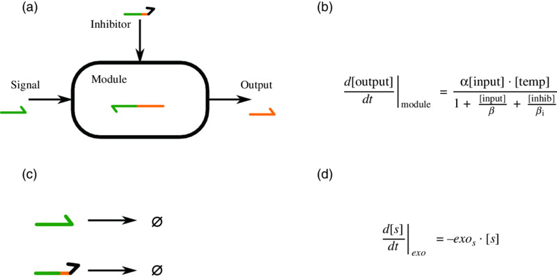
Figure 11.3 (a) Black box representation of a template. (b) The general form of the transfer function for this box, with α the optimal speed of the module, [.] the concentration of DNA compounds, β and βi the Michaelis parameters of the input and inhibitor, respectively. (c) The reactions involving the exonuclease: each unprotected compound (anything but templates) is degraded over time. (d) The contribution of the exonuclease to the equation describing the evolution of the compounds s over time. exos, the activity of the exonuclease with respect to s, usually depends on the length of s. In general, this means that two values are possible, one for signals and one for inhibitors (slightly longer).
This model of the DNA PEN toolbox was first introduced in Padirac et al.’s work on the bistable switch [4]. Because of the simplicity of the equations, large systems can be simulated extremely fast. This propriety was leveraged to evolve complex PEN toolbox systems, requiring thousands of separate evaluations. In this process, interesting patterns were discovered by the algorithm [41] (Figure 11.4).

Figure 11.4 Left: a large evolved system sensing its environment (three nodes at the top) and computing a new internal state. Right: various recurring patterns generated during various runs. One may consider them “standard” subroutines that are combined together to make larger systems.
Applying the principles of this model, we can write the behavior of an autocatalytic template as a single equation:

11.2.3 Internal State of the Templates
The main problem with the previous model is that it does not keep track of the various steps necessary to generate an output. This removes a lot of delays that are actually characteristic of real systems. In fact, the lack of delay makes it harder to design oscillators [3], and probably other systems. Additionally, the previous model makes signal and inhibitor compounds much easier to degrade, as they are never considered to be in a double-stranded state, which would prevent the action of the exonuclease.
For these reasons, we can make a more complex, domain-level model that takes into account all the potential template configurations. The main assumption of such model is that a given signal strand is either completely free or completely double-stranded to its complementary domain. This allows us to abstract away the potential complexity of partially complementary structures as well as the actual transitions from single-stranded to double-stranded into the stability of the sequence, a parameter of the model.
While it is possible to keep the “black box” abstraction for the behavior of templates, the content of the box is much more complex. First of all, we need six variables per template to keep track of the current concentration of all configurations: free template, template with input, template with output, template with both, double-stranded template and inhibited template. The list of all reactions happening with a given template is depicted in Figure 11.5.

Figure 11.5 Left: Reactions related to activation. Non-enzymatic reactions (hybridization and denaturation) are reversible and as such are represented by a double-headed arrow. Enzymatic reactions (polymerization and nicking) are not reversible. Right: Reactions related to inhibition. Because an inhibitor always leave a short toehold on the left and on the right of the template, it is possible for both the input and the output to invade and remove the inhibitor. Note that this is done at a slower speed than hybridization, with a slowdown dependent on the number of free bases [42].
The expression for exonuclease does not change; however, the meaning of s in Figure 11.3(d) is slightly different, as it represents now the concentration of s that is not attached to a template. Note that it is still possible to get back the total concentration of any signal or inhibitor by summing over all configurations that contain it. Note that for an autocatalytic template, the tempboth configuration has to be counted twice, as it contains two copies of the compound.
The set of equation describing an autocatalytic template thus becomes:


In this equation, kduplex represents the (global) hybridization rate, Ks the stability of sequence s, nick, pol and exo the activity of the nickase, polymerase and exonuclease, respectively. A complete explanation of all parameters involved in this model are available elsewhere [35].
11.2.4 Sequence Dependence
Beyond the domain level, we can consider sequence dependence. Taking whole sequences into account might add new possible reactions such as cross-talks. A hybrid solution is to only define the couple of nucleotides at the nicking site, as they are mostly relevant to dangles [43] and stacking [44, 45]. Specifically, Santalucia et al. argues that the nearest-neighbor model is not significantly improved by taking into account bases further away. The full sequence can also be used to check before-hand for cross-talks (including secondary structures, that is, a compound folding onto itself) and to determine a given compound stability.
The hybrid version adds three parameters to each templates: dangle slowdowns to the denaturation of DNA strands, respectively, from the input and output position, and a stacking slowdown to the denaturation in the case both input and output are present. There is also a shared dangle slowdown for inhibitors on their target template, as the base at this position is fixed in the current design. To be more precise, it is part of the recognition site of the nicking enzyme, which means surrounding bases are also fixed. In a design where inhibitors have variable length, a template-specific value should be introduced.
11.2.5 Enzymatic Saturation
While the previous sections explored various level of details for the interactions of DNA molecules, enzymatic activity has been kept as a constant reaction rate. In this section, we explore the impact of adding enzymatic saturation in the model. Enzymatic saturation is the cause for many effects, including winner-take-all effect [35, 46, 47] and robust oscillations [48]. An example of the impact of saturation is shown in Figure 11.6. Keeping track of it adds one variable per enzyme. This comes at a slight computational cost and may affect performances as ODE can become “steep”.

Figure 11.6 A saturation-based oscillator. Left: the topology of the system. Note that both parts are identical. The only symmetry-breaking element is the initial concentrations of the signal compound. Right, top: without saturation, the system can only perform damped oscillations. The green curve has been offset to increase the readability. Right, bottom: when enzymatic saturation is added to the model, the system can oscillate as each side alternatively gets to a high state where the polymerase gets saturated, decreasing the generation of inhibitor for the other side.
Saturation is done by the substracts; so the first step is to identify which substracts are valid. See Figure 11.7. A few design tricks, such as using U instead of T in nickase recognition site of the output area of a template, can remove some of those substracts or reduce their impact [13].

Figure 11.7 Example of substracts that can be considered to saturate the various enzymes present in the system.
For all models, the exonuclease term becomes:

where Vm, exo is the maximum theoretical rate and Ksm, exo the Michaelis constant for the compounds s. Note than in our model Vm, exo is independent of s and Ksm, exo can only take one of two values, depending on whether s is an inhibition compound or not.
For the polymerase and nickase, since all substracts are taken into account at the second level of detail, that of templates internal states, saturation can be easily expressed.
The polymerase activity is separated in two terms: pol for templates with input alone and poldispl in the case where both input and output are present. We consider that the polymerase does not interact noticeably with other states of the template.

Note that Vm, displ depends on the length of the output. It has been argued that signal strands are short enough to not be a bother (no slowdown) while inhibitor have been measured to have a slowdown of 0.2 with the Bst polymerase [4]. The nickase term is simpler. We consider that only fully double stranded templates can capture this enzyme, yielding:

For the simplest model presented here, since we are considering that hybridization /denaturation reactions are near equilibrium, we can estimate the concentration of the various substracts of the enzymes. Additionally, pol and nick should give us a more explicit expression of α in Section 11.2.
If Ks represents the equilibrium constant of the hybridization of the DNA compound s with its complementary ![]() , then the amount of duplexed DNA
, then the amount of duplexed DNA ![]() is
is
By taking the system of reactions from Figure 11.5 and assuming equilibrium for hybridization/denaturation pairs, in the simplified case where there is no inhibitor, we find:

This yields αtemp = pol · K− 1in and ![]() .
.
In the presence of inhibitor, and under the assumption that it only reacts with free templates, we get a slightly more complicated formula:

Note that the equation now depends on [out](t). Also note that ![]() is only approximately constant for [out](t) ≪ Kout.
is only approximately constant for [out](t) ≪ Kout.
In the case of the saturation of the nicking enzyme, we want to find the fraction of all templates which are double-stranded.

Note that this equation contains nick. However, the activity in the formula should the one at the previous time step of the simulation. We might also want to add other potential substrates, such as templates with output or templates with both input and output.
In the case of the saturation of the polymerase, we want to know the fraction of all templates with input. Going through the same calculation as for the nickase, we get:

This yields the actual enzyme activities
were both base activities and Michaelis parameter Kenzyme can be determined experimentally.
11.3 RELATED WORK
In this section, we cover the previous attempts to automate the design of genetic or chemical circuits by using EC techniques.
Initially, Francois and Hakim [20] used a mutation-only genetic algorithm (GA) to evolve both the structure and reaction rates of genetic regulatory networks in the form of an idealized abstraction. The discovered circuit designs were shown to be promising, as they were functionally relevant to the organization of known biological networks. The efficiency of evolutionary computations on this initial attempt, despite the simplicity of the evolutionary scheme, encourages later research on such problems. As a result, Fujimoto et al. [21] used a similar algorithm to evolve gene regulatory networks that produce striped patterns of gene expression. The evolved networks were analyzed and classified into three categories which reproduce various segmentation strategies observed among arthropods. Likewise, an algorithm with only structural mutations were used by Kobayashi et al. [22] to discover genetic networks that display steady periodic oscillations with a given temporal period. Another simple genetic algorithm without crossover was used by Deckard and Sauro [23] to evolve chemical reaction networks with specific signal processing capabilities. As reported in their work, crossover provided worse performance. Later, Deckard and Sauro’s work was extended by Paladugu et al. [24] to successfully evolve oscillators, bistable switches, homeostatic systems, and frequency filters. Interestingly, crossover was still not included for the possibility of being disruptive.
When it comes to difficult problems or complex models that require heavy computation, simple GAs with mutation as the only genetic operator are not efficient enough, and several workarounds have been suggested. One example is the study carried out by Marchisio and Stelling [25], in which the structure design and parameter optimization are separated from each other. For a given truth table that specifies a circuit’s input–output relations, their algorithm generates and ranks several possible circuit schemes without any optimization procedure. Then, only the most feasible solution undergoes a parameter optimization aiming for reliable performance in actual wet experiments. This method relies on the existence of a rational solution, which cannot always be expected, especially in complex tasks. Moreover, the most feasible solution might require an accurate combination of both structure and parameters, advocating for their co-evolution. Cao et al. [26] also highlighted this issue, and efficiently addressed it with a nested evolutionary algorithm. Their algorithm first identifies the sequential structure of the target system and then optimize parameters of the selected modules. Notably, there are several works that simply freeze the structure, and only optimize parameters with the use of an efficient Evolution Strategy (ES), for example, the work of Jin and Sendhoff [27], and Hallinan et al. [28].
A complete GA, including mutation, elitist selection, and crossover, was introduced by Drennan and Beer [29] to successfully evolve the genetic regulatory networks that express proteins in an oscillatory manner similar to a repressilator [49]. In their algorithm, pseudo-DNA sequences are used directly as individuals’ encoding and genetic operations are applied in a pseudo-biological way. Because these genetic operators are applied at the sequence level of the genomes while the network graph is encoded by a matrix, there is a high probability that connection will be broken in genetic operators, making it hard to pass on connectivity innovation to later generations. This make the approach inappropriate for problems that require precise combination of connections [31, 32].
Interestingly, on the evolution of a different network structure—the artificial neural network (ANNs)—an algorithm called NEAT [31] has been proposed to efficiently solve the co-evolution of the structure and parameters, and showed better performance than the best fixed topology methods on challenging problems. The increased efficiency has been ascribed to an effective crossover strategy and structural innovation protection, combined with a parsimonious addition of new nodes. All the previous EA approaches for GRN avoided using crossover for the reason that meaningful structural crossover strategies are not obvious and worse performance is usually experienced when crossing over non-homologous networks. Because GRNs and ANNs can both be represented as graphs, we reasoned that it might be possible to apply NEAT’s strategies to GRN’s in silico evolution, with a potentially large improvement in search efficiency. The next section will describe how we adapt NEAT to come up with a new algorithm, namely ERNe, for the evolution of realistic molecular circuits targeting a given dynamic function.
11.4 FRAMEWORK FOR EVOLVING REACTION NETWORKS (ERNE)
ERNe is an efficient derivative of the NeuroEvolution of Augmenting Topologies (NEAT) algorithm [31] directed at the evolution of biochemical systems or molecular programs. The main differences between ANN and reaction networks are the addition of inhibition links and biochemical parameters. Therefore, as an extension of NEAT, ERNe encoding allows representation of inhibition, and has added parameters. In addition, ERNe’s mutation and crossover operators are also modified from the original NEAT. For better understanding of ERNe algorithm, this section described in detail the encoding, the genetic operators for mutation and crossover, and the speciation process.
11.4.1 Encoding
Similar to NEAT, our genome consists of sequence genes and template genes. However, each sequence gene can represent either a signal sequence or an inhibiting sequence in the system, and consists of a sequence name, a kinetic parameter, and an initial concentration. Each template gene represents a template sequence in the system, and specifies the from-node, the to-node, the template concentration, an enable bit that indicates whether or not the template is enabled, and an innovation number to help align corresponding template genes. This innovation number is very important for the implementation of the crossover and speciation. For assigning innovation number to a template gene, we use the following rules: during the evolution, whenever a template is added to a system, we check if that specific link exists in the evolution history (using the from-node and the to-node fields), in which case it takes the original linkś innovation number. Otherwise, the next available innovation number will be assigned to the template gene. As for naming newly added nodes, the following mechanism is used: we map node names with the way they are created, for example, an entry A→A to B shows that whenever a new node is added in the middle of the template A→A, it must be named B. An example of the genetic encoding is shown in Figure 11.8.

Figure 11.8 A graph representation and corresponding ERNe encoding of the Oligator. Nodes represent sequences while arrows represent templates; bar-headed arrows represent inhibition. a and b are signal sequences, whereas the green node Iaa is an inhibiting sequence; it inhibits the template a→a (i.e., the self-activation of a). The system has three sequences and three templates. Thus, there are three node genes and three connection genes in its ERNe encoding.
11.4.2 Mutations
In our framework, mutations can be applied to change both the parameters and the network structure. We have the following mutation rules: parameter only, disable template, switch template, add sequence, add activation, and add inhibition. Their relationship is shown in Figure 11.9. Which mutation to be applied is defined based on some probability parameters that can be set before running.

Figure 11.9 Different types of mutation used in ERNe. Note that although mutate disable template and mutate switch template belong to parameter mutation, they actually change the structure as well.
In parameter mutation, every parameter has a probability to be mutated to a new value calculated as:
where rand are standard normal deviates. If the new value of a template concentration is above zero and below a threshold, it has a probability to be disabled. In this case, we call it disable template mutation. If that value is below zero, a switch template mutation happens. An example of switch template mutation is shown in Figure 11.10. In this example, assume template b→a’s concentration is mutated to a value below zero. The following changes will be applied to the system:
- Disable template b→a.
- Search for any template that create a, if there is no such template, add the template a→a. In this example, a→a is found and selected.
- Add the inhibiting sequence to the selected template a→a, Iaa.
- Add the template from b to Iaa, b→Iaa.

Figure 11.10 Switch template mutation. The template b→a is disabled, an inhibition node Iaa is added, then a template b→Iaa is added with a new innovation number.
Because the parameter is mutated based on normal distribution, a template that has the concentration closer to zero has higher chance to be disabled, or be switched. These mutations are based on the idea that, once a connection has no meaning (template concentration close to zero), it should be removed (disabled), or changed to a reverse polarity.
In add sequence mutation, a new signal sequence is added to the system. There are several ways to do so as described in Figure 11.11. The first way is to select an existing template, split it and place the new sequence in the middle. The second way is to add a new sequence that is connecting to itself to inhibit an existing template. In the third way, the added sequence is connected to itself and activates an existing sequence.

Figure 11.11 Add sequence mutation, with (a) a sequence c added in the middle of existing template a→a, (b) a sequence c added to inhibit template a→b, and (c) a sequence c is added to activate sequence b.
In add activation mutation, two sequences are chosen randomly with the condition that there is no connection between them. Then, a new template is added connecting the two selected sequences. This process is shown in Figure 11.12.

Figure 11.12 Add activation mutation. The template b→b is added.
The add inhibition mutation’s example is described in Figure 11.13. First, two simple sequences are chosen, and the template connecting those two simple sequences is disabled (if it exists). In the example, two sequences b and a are chosen and template b→a is disabled. Next, a random template that is generating a is selected (a→a in the example). Then, a new inhibition node is added to inhibit the selected template (Iaa). Finally, the mutation adds the template b→Iaa, completing the module in which sequence b is inhibiting the creation of sequence a.

Figure 11.13 Add inhibition mutation. The template b→a is disabled, an inhibiting sequence Iaa is added, and a template b→Iaa is added.
In the mutation, whenever a template is added to the system, we have to check whether that template innovation exists in the evolution history or not. In order to keep track of that, we use a list to map the template to innovation number. For example, a→a is mapped to 1; a→b is mapped to 2. Thus, in the future, if the template a→b is somehow added to a system, its innovation number is set to 1, whereas a new template that does not exist in the map will be given the next available innovation number. This new map is then added to the list. This innovation number plays an important role in the implementation of the crossover and speciation.
11.4.3 Crossover
The ERNe encoding and the use of innovation number make crossover straightforward. The template genes in both parents are lined up in the order of innovation number and aligned, and crossover techniques such as one-point and two-point crossover can be applied. Figure 11.14 shows an example of two different individuals’ two-point crossover, in which a new topology can be efficiently constructed. We then need to decide how to create node genes for the child. Currently, we are using a simple way: we start with an empty list of node genes, and for each connection gene in the child, we add the involved nodes (from-node and to-node)—with the parameters of corresponding nodes in the parent the connection is inherited from—to the list if no such node is already there.

Figure 11.14 Two-point crossover of the two individuals Parent 1 and Parent 2. The template genes are lined up in the order of innovation number. The red lines show the two crossover points. The child takes the gene number 1, 2, 5, 6, 7, and 8 from Parent 1, and gene number 3 and 5 from Parent 2. As a result, we have a new topology that has some parts of both parents.
11.4.4 Speciation
In complex optimization problems, topological innovations are very hard to be preserved. The first reason is that smaller structures tend to optimize faster than larger structure. Moreover, adding new nodes and connections to the system usually decreases the fitness initially. Thus, newly discovered structures are hard to survive more than one generation, even though the innovations they represent might be crucial toward solving the task in the end [31]. We will divide the population into species so that individuals that have similar topologies will be put in same species. Individuals then only have to compete within their own niches instead of with the whole population. This way, topological innovations are protected and have time to optimize. Our speciation is similar to NEAT as we also use a compatibility distance δ calculated as:
where M is the number of mismatched genes and N is the number of genes in the larger genome. If δ is below the speciation threshold δt, we say that the two individuals can be put in the same species. For every individual created in the current generation, we try to find its species by looking at all the species from all the generations, with higher priority to more recent species. If no suitable species is found, a new species is added containing the individual.
Every species at the current generation is then assigned a different number of offspring in proportion to the average fitness of its individuals. This mechanism ensures that individuals in the same species must share the fitness of their niche. Therefore, a species is considered better if it has higher average fitness from all the individuals. We also implement a capping mechanism to prevent some temporal good species from growing too fast and taking all the population space. That is, from a generation to the next one, each species can grow to at most 10% of the whole population plus its current population. In order to control the number of species at each generation, we implemented a dynamic adjustment of speciation threshold so that the number of species will move toward a specific target Ns:
ε is called the modification step.
11.5 ERNE FOR THE DISCOVERY OF OSCILLATORY SYSTEMS
In its appearance [32], ERNe was demonstrated by evolving credible biochemical answers to challenging autonomous molecular problems: in vitro batch oscillatory networks that match specific oscillation shapes. Statistical results clearly show that significant improvements in performance were obtained over other approaches. In this section, we report ERNe’s application to two other interesting oscillatory problems: fast-strong oscillator, and robust-fast-strong oscillator.
11.5.1 Fast-Strong Oscillator
In this experiment, the target solution is a PEN DNA toolbox system that can oscillate with high amplitude and frequency. The tracking signal sequence is the sequence a, and the fitness is given as follows:
where amplitude is the concentration of the tracking sequence at its first peak after some skip time, step_size is the difference in time between the first peak and the second peak, and limitcycle is calculated as follows:

where lastPeakAmplitude is the concentration of the tracking sequence at its last peak within observation time (see Figure 11.15 for better understanding of the terms).

Figure 11.15 How to define first peak, second peak, and last peak.
From the fitness function, it is clearly seen that we are looking for a system that should have the highest amplitude, the highest limitcycle (capped at 1), and the lowest step size.
For this problem, the ERNe algorithm was run 100 times using the same settings shown in Table 11.1. The best individuals from the runs were then taken for analysis. Interestingly, all the solutions are based on a long oligator [32], having the tracking signal sequence a as the autocatalysis (Figure 11.5.1). The solutions are different in the length of feedback loop (i.e., number of nodes in the feedback loop), varying from 4 to 9. We will investigate how this length affects the fitness.

Figure 11.16 Two derivatives of the long oligator, having tracking sequence as the first (a), and the last (b) nodes of the feedback loop.
Table 11.1 Parameters used in experiments
| General parameters | |
| Population size | 200 |
| Number of generations | 100 |
| Selection method | Tournament (size 5) |
| Crossover technique | One-point crossover |
| Speciation parameters | |
| Preferred number of species | 10 |
| Starting speciation threshold | 0.6 |
| Minimum speciation threshold | 0.1 |
| Speciation modification step ε | 0.03 |
| Crossover and mutation parameters | |
| P (mutation only) | 0.5 |
| P (interspecies mating) | 0.01 |
| P (mutation after crossover) | 0.75 |
| Mutation parameters | |
| P (parameter only) | 0.9 |
| P (single gene mutation) | 0.8 |
| P (structure-add node) | 0.2 |
| P (structure-add activation) | 0.2 |
Figure 11.17 shows the distribution of fitness over feedback loop’s length. It can be seen that solutions with four nodes in their feedback loop has the highest median fitness. However, only 3/100 of the runs finished finding these solutions. The largest proportion of the runs (38/100), and the highest fitness solution (1.97) fall into the group with feedback loop length of 7. The number of solutions for the group with 5, 6, 7, and 9 nodes in their feedback loop are 10, 17, 24, and 8, respectively. The median fitness for these group are not significantly different.

Figure 11.17 Fitness plotted against number of nodes in the feedback loop.
As we have a closer look at all the solutions, their limit cycles are all equal to or very close to the capped value of 1. Thus, it is the amplitude and step size that contribute to the fitness. For better understanding of the relationship between these behaviors and the feedback loop length, we have two additional plots, showing the amplitudes (Figure 11.18) and step sizes (Figure 11.19) over the feedback loop length. It can be clearly seen that, step size increases with the length of the feedback loop. As for the amplitude, we observe a similar thing, with the exception of the group of length four. This group can reach as high an amplitude as the group of length six, but cannot compete with the group of length seven or above.

Figure 11.18 Amplitudes plotted against number of nodes in the feedback loop.

Figure 11.19 Step sizes plotted against number of nodes in the feedback loop.
11.5.2 Robust-Fast-Strong Oscillatior
Our ultimate goal is for finding direct candidates for the wet experiment. Thus, robustness is also an important factor. Similar to previous experiment, we want a PEN DNA toolbox system that can oscillate with high amplitude and frequency. In this experiment, however, we also require the system to be robust. For a solution, we generate 30 systems which are the noisy version of the solution, simply by mutating all its sequences’ parameters using the parameter mutation operation. Then, the fitness of a solution is defined as:
where amplitudei, limitcyclei, and stepsizei are the amplitude, limitcycle, and step_size (see previous section) of the ith noisy version of the solution.
This way of evaluating the robustness is efficient, but it is also costly in computational power. For this reason, we only have the ERNe algorithm run for five times using the settings shown in Table 11.1. Again, all runs converged to a topology based on the long oligator of length five, this time having the tracking signal sequence positioned in the end of the feedback loop (Figure 11.5.1).
11.6 DISCUSSION
The results reported for the fast-strong oscillator shows that high amplitude can be obtained by simply increasing the length of the feedback loop. However, longer feedback loop tends to have slower oscillation. As a result, it is non-trivial to know the design of a best fast-strong oscillator. It can be concluded from our study that a long oligator starting from the tracking signal sequence with the length of the feedback loop between 4 to 9—with their parameters optimized—can do the job fairly well. From the plot shown in Figure 11.17 also, it can be seen that fitness slightly improves with the complexity, but we never found a solution with the length of feedback loop greater than nine. It means that the bloating problem is controlled well with ERNe without any need to implement fitness penalty to the complexity.
Besides the length of the feedback loop, the solutions are also different in the way side branches are forged. At the moment, it is impossible for us to know in a systematic way how such branches contribute to the fitness. Instead, we take the best solution (Figure 11.20a) with fitness of 1.97 (amplitude is 149.70 nm and step size is 76 min) and remove its side branches, to form the topology in Figure 11.20b. Its new observed fitness dropped significantly to 0.77 (amplitude is 83.88 nm and step size is 108 min). This shows that the side branches contribute greatly to both the amplitude and frequency, therefore boosting the fitness score.

Figure 11.20 Original (a) and pruned (b) versions of the best solution for the Fast-strong oscillator.
It is also interesting that we found the completely different topology as the solution for the robust-fast-strong oscillation. This means that robustness can not be expected to be easily compatible with fast and strong characteristics in oscillators. Nevertheless, there are still some difficulties in analyzing the results coming out of the ERNe algorithm. We know that they are most feasible candidates for the actual wet experiments, but we do not know by which mechanism could they obtain the desired behavior. We believe that, by actually implementing them we could get some insights.
Another thing we would like to discuss is that, even though ERNe is designed for the evolution of biochemical reaction networks, it can be used on GRNs without any difficulties. Indeed, the ERNe encoding can be used directly to encode the structure and parameters of GRNs, and ERNe’s crossover and speciation can also be used directly. The mutation rules, though, should be redefined, as in our previous paper [32] we discovered that the physical nature of the information processing medium should be taken into account in the definition of relevant mutation operators. In the future, we would like to explore the mixed use of the model levels, the use of local search [50], multi-objective optimization [51, 52], and automatic parameter tuning [53, 54].
11.7 CONCLUSION
In this chapter, we introduced an up-to-date research in in vitro molecular programming: a GRN-inspired system called the PEN DNA Toolbox. One of its advantages is that it offers simulation in various levels of details, with the highest level accurate enough to enable direct transfer from in silico design to in vitro wet experiment. Using the most efficient technique which is the ERNe algorithm, we discovered some designs for the two interesting problems: fast-strong oscillator, and robust-fast-strong oscillator. The study clearly shows that the amplitude and the frequency of oscillations cannot be expected at the same time, and that a long oligator with feedback loop length 4 to 9 should be best for the job. In the future, we would like to explore the use of mixed model levels, the use of local search [50], multi-objective optimization [51, 52], and automatic parameter tuning [53, 54].
REFERENCES
- F. Lienert, J. J. Lohmueller, A. Garg, and P. A. Silver, “Synthetic biology in mammalian cells: next generation research tools and therapeutics,” Nature Reviews Molecular Cell Biology, 15(2), 95–107 (2014).
- K. Roberta, “Five hard truths for synthetic biology,” Nature, 463(7279), 288–290 (2014).
- K. Montagne, R. Plasson, Y. Sakai, T. Fujii, and Y. Rondelez, “Programming an in vitro DNA oscillator using a molecular networking strategy,” Molecular Systems Biology, 7(1) (2011).
- A. Padirac, T. Fujii, and Y. Rondelez, “Bottom-up construction of in vitro switchable memories,” Proceedings of the National Academy of Sciences, 109(47), E3212–E3220 (2012).
- L. Qian, E. Winfree, and J. Bruck, “Neural network computation with DNA strand displacement cascades,” Nature, 475, 368–372 (2011).
- A. Padirac, T. Fujii, and Y. Rondelez, “Nucleic acids for the rational design of reaction circuits,” Current Opinion in Biotechnology, 24(4), 575–580 (2012).
- M. N. Stojanovic and D. Stefanovic, “A deoxyribozyme-based molecular automaton,” Nature Biotechnology, 21, 1069–1074 (2003).
- J. Kim, K. S. White, and E. Winfree, “Construction of an in vitro bistable circuit from synthetic transcriptional switches,” Molecular System Biology, 2(68) (2006).
- G. Seelig, D. Soloveichik, D. Y. Zhang, and E. Winfree, “Enzyme-free nucleic acid logic circuits,” Science, 314(5805), 1585–1588 (2006).
- T. Fujii and Y. Rondelez, “Predator-prey molecular ecosystems,” ACS Nano, 7(1), 27–34 (2013).
- A. Padirac, T. Fujii, A. E. Torres, and Y. Rondelez, “Spatial waves in synthetic biochemical networks,” Journal of the American Chemical Society, 135(39), 14586–14592 (2013).
- D. Soloveichik, G. Seelig, and E. Winfree, “DNA as a universal substrate for chemical kinetics,” Proceedings of the National Academy of Sciences, 107(12), 5393–5398 (2010).
- A. Baccouche, K. Montagne, A. Padirac, T. Fujii, and Y. Rondelez, “Dynamic DNA-toolbox reaction circuits: a walkthrough,” Methods, 67(2), 234–249 (2014).
- S. Tavazoie, J. D. Hughes, M. J. Campbell, R. J. Cho, G. M. Church, “Systematic determination of genetic network architecture,” Nature Genetics, 22(3), 281–285. (1999).
- T. I. Lee, N. J. Rinaldi, F. Robert, D. T. Odom, Z. Bar-Joseph, G. K. Gerber, N. M. Hannett, C. T. Harbison, C. M. Thompson, I. Simon, J. Zeitlinger, E. G. Jennings, H. L. Murray, D. B. Gordon, B. Ren, J. J. Wyrick, J-B Tagne, T. L. Volkert, E. Fraenkel, D. K. Gifford, R. A. Young, “Transcriptional Regulatory Networks in Saccharomyces cerevisiae,” Science, 298(5594), 799–804 (2002).
- D. Peer, A. Regev, G. Elidan, and N. Friedman, “Inferring subnetworks from perturbed expression profiles,” Bioinformatics, 17(Suppl 1), S215–S224 (2001).
- K. Basso, A. A. Margolin, G. Stolovitzky, U. Klein, R. Dalla-Favera, and A. Califano, “Reverse engineering of regulatory networks in human B cells,” Nature Genetics, 37(4), 382–390 (2005).
- N. Kasabov, “Knowledge-based neural networks for gene expression data analysis, modelling and profile discovery,” Drug Discovery Today: BIOSILICO, 2(6), 253–261 (2004).
- Z. S. Chan, N. Kasabov, and L. Collins, “A two-stage methodology for gene regulatory network extraction from time–course gene expression data,” Expert Systems with Applications, 30(1), 59–63 (2006).
- P. Francois and V. Hakim, “Design of genetic networks with specified functions by evolution in silico,” Proceedings of the National Academy of Sciences, 101(2), 580–585 (2004).
- K. Fujimoto, S. Ishihara, and K. Kaneko, “Network evolution of body plans,” PLOS ONE, 3(7) (2008).
- Y. Kobayashi, T. Shibata, Y. Kuramoto, and A. Mikhailov, “Evolutionary design of oscillatory genetic networks,” European Physical Journal B, 76, 167–178 (2010).
- A. Deckard and H. M. Sauro, “Preliminary studies on the in silico evolution of biochemical networks,” ChemBioChem, 5(10), 1423–1431 (2004).
- S. R. Paladugu, V. Chickarmane, A. Deckard, J. P. Frumkin, M. Mc-Cormack, and H. M. Sauro, “In silico evolution of functional modules in biochemical networks,” Systematic Biology (Stevenage), 153(4), 223–235 (2006).
- M. A. Marchisio and J. Stelling, “Automatic design of digital synthetic gene circuits,” PLoS Computers in Biology, 7(2), (2011).
- H. Cao, F. J. Remoro-Campero, S. Heeb, M. Cmara, and N. Krasnogor, “Evolving cell models for systems and synthetic biology,” Systems and Synthetic Biology, 4(1), 55–84 (2010).
- Y. Jin and B. Sendhoff, “Evolving in silico bistable and oscillatory dynamics for gene regulatory network motifs,” IEEE Congress on Evolutionary Computation, 386–391 (2008).
- J. S. Hallinan, G. Misirli, and A. Wipat, “Evolutionary computation for the design of a stochastic switch for synthetic genetic circuits,” Conference Proceedings of the IEEE Engineering in Medicine and Biology Society, 768–774 (2010).
- B. Drennan and R. Beer, “Evolution of repressilators using a biologically-motivated model of gene expression,” Artificial Life X: Proceedings of the Tenth International Conference on the Simulation and Synthesis of Living Systems, 22–27 (2006).
- A. H. Chau, J. M. Walter, J. Gerardin, C. Tang, and W. A. Lim, “Designing synthetic regulatory networks capable of self-organizing cell polarization,” Cell, 151(2), 320–332 (2012).
- K. O. Stanley and R. Miikkulainen, “Evolving neural networks through augmenting topologies,” Evolutionary Computation, 10(2), 99–127 (2002).
- Q. H. Dinh, N. Aubert, N. Noman, T. Fujii, Y. Rondelez, and H.Iba “An effective method for evolving reaction networks in synthetic biochemical systems,” IEEE Transactions on Evolutionary Computation, 19 (3), 374–386 (2015).
- L. Qian and E. Winfree, “Scaling up digital circuit computation with DNA strand displacement cascades,” Science, 332(6034), 1196–1201 (2011).
- R. Plasson and Y. Rondelez, “Synthetic biochemical dynamic circuits,” Multiscale Analysis and Nonlinear Dynamics: From Genes to the Brain, p. 113–145 (2013).
- N. Aubert, C. Mosca, T. Fujii, M. Hagiya, and Y. Rondelez, “Computer-assisted design for scaling up systems based on DNA reaction networks,” Journal of the Royal Society Interface, 11(93), (2014).
- P. D. Dans, A. Zeida, M. R. Machado, and S. Pantano, “A coarse grained model for atomic-detailed DNA simulations with explicit electrostatics,” Journal of Chemical Theory and Computation, 6(5), 1711–1725 (2010).
- T. E. Ouldridge, “Springer Theses: Coarse-Grained Modelling of DNA and DNA Self- Assembly,” Springer, (2012).
- N. R. Markham and M. Zuker, “Dinamelt web server for nucleic acid melting prediction,” Nucleic Acids Research, 33(Suppl 2), W577–W581 (2005).
- P. Yakovchuk, E. Protozanova, and M. D. Frank-Kamenetskii, “Base-stacking and base-pairing contributions into thermal stability of the DNA double helix,” Nucleic Acids Research, 34(2), 564–574 (2006).
- Y. Bansho, N. Ichihashi, Y. Kazuta, T. Matsuura, H. Suzuki, and T. Yomo, “Importance of parasite RNA species repression for prolonged translation-coupled RNA self-replication,” Chemistry and Biology, 19(4), 478–487 (2012).
- N. Aubert, Q. H. Dinh, M. Hagiya, H. Iba, T. Fujii, N. Bredeche, and Y. Rondelez, “Evolution of cheating DNA-based agents playing the game of rock-paper-scissors,” Advances in Articial Life, ECAL, 12, 1143–1150 (2013).
- D. Y. Zhang and E. Winfree, “Control of DNA strand displacement kinetics using toehold exchange,” Journal of the American Chemical Society, 131(47), 17393–17314 (2009).
- S. Bommarito, N. Peyret, and J. SantaLucia Jr., “Thermodynamic parameters for DNA sequences with dangling ends,” Nucleic Acids Research, 28(9), 1929–1934 (2000).
- V. A. Vasiliskov, D. V. Prokopenko, and A. D. Mirzabekov, “Parallel multiplex thermodynamic analysis of coaxial base stacking in DNA duplexes by oligodeoxyribonucleotide microchips,” Nucleic Acids Research, 29(11), 2303–2313 (2001).
- D. V. Pyshnyi and E. M. Ivanova, “The influence of nearest neighbors on the efficiency of coaxial stacking at contiguous stacking hybridization of oligodeoxyribonucleotides,” Nucleosides, Nucleotides and Nucleic Acids, 23(6–7), 1057–1064 (2004).
- J. Kim, J. Hopfield, and E. Winfree, “Neural network computation by in vitro transcriptional circuits,” Advances in Neural Information Processing Systems, p. 681–688 (2004).
- A. J. Genot, T. Fujii, and Y. Rondelez, “Computing with competition in biochemical networks,” Physical Review Letters, 109(20) (2012).
- Y. Rondelez, “Competition for catalytic resources alters biological network dynamics,” Physical Review Letters, 108(1) (2012).
- M. B. Elowitz and S. A. Leibler, “Synthetic gene oscillatory network of transcriptional regulators,” Nature, 403, 335–338 (2000).
- R. Storn and K. Price, “Differential evolution - a simple and efficient heuristic for global optimization over continuous spaces,” Journal of Global Optimization,11(4), 341–359 (1997).
- K. Deb, “Multi-Objective Optimization Using Evolutionary Algorithms,” NJ: Wiley, (2001).
- A. Warmflash, P. Francois, and E. D. Siggia, “Pareto evolution of gene networks: an algorithm to optimize multiple fitness objectives,” Physics and Biology, 9(5) (2012).
- A. E. Eiben, R. Hinterding, and Z. Michalewicz, “Parameter control in evolutionary algorithms,” IEEE Transactions on Evolutionary Computation, 3(2), 124–141 (1999).
- A. E. Eiben and S. K. Smit, “Parameter tuning for configuring and analyzing evolutionary algorithms,” Swarm and Evolutionary Computation, 1(1), 19–31 (2011).