8.1 INTRODUCTION

Systems biology is an evolving field that allows holistic analysis by uncovering the system-level principles of a biological system. According to Brazhink et al. [6], a biological system can be visualized as a multi-layered network of different processes. An abstract view of such a system, shown in Figure 8.1, considers the processes as involving variables such as metabolites, proteins, and genes in separate layers. However, in reality, the variables in each layer interact not only with the variables in the same layer but also with the variables in other layers. In most of these underlying interactions, genes play an important role in carrying out the complex biochemical interactions. Thus, a gene regulatory network (GRN) acquires significance as it can reveal the underlying biological processes of living organisms, and provide new insights into the causes of complex diseases or for designing new drugs [16]. As a functional circuitry of a living organism, GRN exhibits the regulatory relationships

among genes of a cellular system. The responses of genes are represented by their expression profiles, which are captured during the deoxyribonucleic acid (DNA) microarray experiments [43]. A GRN (also referred to as genetic network or gene network) represents the relationship among genes of a genome. In an equivalent graph representation of an N-gene GRN, a gene is shown to be regulated by all N genes, including the self-regulation. However, investigations by Bolouri and Davidson [5] show that, on average, a gene can be regulated typically by four to eight other genes. Figure 8.2(a) shows a GRN of 10 genes having 11 regulations, while Figure 8.2(b) shows a large-scale GRN of 100 genes where, as we can easily realize, it is extremely difficult to count the number of regulations (= 193) from this form of graphical representation.

8.1.1 Significance of Inferring Large-Scale Gene Regulatory Networks

A GRN plays a crucial role in controlling various mechanisms inside a cell. Understanding the interactions among genes helps in understanding the inner details of

cells, and the ability to accurately reconstruct a GRN serves this important objective. Among various available computational techniques, evolutionary algorithms (EAs) are commonly applied for optimizing GRNs during reverse engineering, that means, to optimally learn the model parameters used to represent a network. Since, real-life GRNs consist of thousands of genes, effective and efficient techniques are required to reconstruct the GRN accurately in a reasonable computational time frame.

Reverse engineering GRN is the process of identifying genetic interactions using time-series data with an appropriate mathematical model. These gene-expression data go beyond a generic view of the genome and differentiate between genes within (i) different tissues of the same organism and (ii) different states of the cells in the same tissue. With the advent of cutting-edge technologies for gene profiling, massive amounts of biological data are now available to researchers enabling them to unravel the underlying transcriptional regulations in gene circuits using model-based identification methods.

Thus, reconstructing the genome-wide GRN is a crucial step in uncovering the complete biochemical networks of cells. A GRN helps in understanding interactions at the cellular level and has immense potential for application in genetic engineering. Moreover, knowledge about GRNs provides valuable evidence for the therapeutic studies of complex diseases [3, 38]. Since a real-life GRN consists of thousands of genes, both the model and the method should be robust enough to cope with that amount of genes. However, the model of our particular interest, that is, the S-system model, is currently suitable for modeling small-scale GRN of 5–20 genes and medium-scale GRN having up to 40–50 genes. Hence, inferring a GRN with the S-system model having a large number of genes (say, more than 50) can be designated as large-scale GRN modeling. Such large-scale modeling requires suitable technique from both modeling and optimization methodology perspectives.

8.2 REVERSE ENGINEERING GRN WITH S-SYSTEM MODEL AND EVOLUTIONARY COMPUTATION

Reverse engineering a GRN as an optimization problem depends not only on selecting an appropriate model, but also on the use or development of a suitable optimization method. Furthermore, the performance of the optimization method is also significantly reliant on the nature of the data, noise level present in the data, sampling time, and the type of regulations. This section is devoted to describing the details of different variants of the S-system model for representing GRNs and efficient optimization methods.

8.2.1 S-System Model

The interaction among the components (e.g., metabolites, genes, and proteins) is nonlinear in nature. Therefore, a nonlinear model is more appropriate for modeling nonlinear processes of GRNs [18, 4, 50, 8]. S-system model, a particularly well-established nonlinear model [41], is capable of capturing various dynamics of the complex regulations. Moreover, the S-system is able to represent the regulations of both production and degradation phases, while the other models can only represent the interactions of the production phase. The S-system has been considered as an excellent balance between model complexity and mathematical tractability; it is complex enough to represent a wide range of dynamics, yet is simple enough to allow certain analytical studies.

The S-system, with a set of tightly coupled nonlinear differential equations, is among the best known nonlinear differential-equation-based models for GRNs. These advantages have led to the successful application of this model to the analysis of biochemical networks [11, 12, 23, 26, 40, 53].

8.2.1.1 Canonical S-System Model

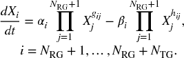
The S-system model, proposed by Savageau [41], is a well-known system for biochemical networks and has mainly attracted attention for GRN inference in the last decade [23, 26, 30]. The S-system approach is found to be both promising and challenging for GRN modeling. For an N-gene network, the component processes are characterized by the following power-law-based S-system equation:

(8.1)

where Xi is the expression level of ith gene. Non-negative parameters αi and βi are called rate constants, and real-valued exponents gij and hij are referred to as kinetic orders. If gij = 0, it implies that there is no activation or inhibition from Gene-j to Gene-i. If gij > 0, Gene-j activates Gene-i and if gij < 0, Gene-j inhibits Gene-i. Compared to gij, the term hij has an opposite effect on the genes i and j, that is, for hij > 0, Gene-j inhibits Gene-i and if hij < 0, Gene-j activates Gene-i. The term αi∏Xgijj models the process of ribonucleic acid (RNA) synthesis, while the term βi∏Xhijj models the process of RNA degradation. The set of parameters that define the S-system model is given as θ = {α, β, g, h}. To infer a GRN of N genes using the S-system model, 2× N(N + 1) parameters must be estimated. Thus, to reverse engineer a small network of 5 genes (N = 5), we need to estimate 2 × 5(5 + 1) = 60 parameters in total, with 12 parameters representing each gene. An investigation of the computational time demonstrates that, in the optimization task for solving tightly coupled S-system model, 95% of the total optimization time is consumed by the numerical integration operation [54]. In order to deal with the problem of high dimensionality and computation complexity for solving S-system equations, different decoupling approaches have been applied to decompose the canonical system into smaller problems.

8.2.1.2 Decoupled S-System Model

As mentioned in Section 8.2.1.1 regarding the computational complexity of canonical S-system modeling, to overcome these limitations, a decoupled system has been proposed by Maki et al. [30]. The decoupled system divides the given problem into N sub-problems, each having 2 × (N + 1) number of parameters. In the ith sub-problem, corresponding to ith gene, the parameter set θ_i = {α_i, β_i, g_ij, h_ij} is estimated by solving the decoupled S-system equation:

(8.2)

For solving Equation (8.2), Y_{i = j} is obtained by numerical integration, whereas Y_{i ≠ j} is obtained by pre-calculations directly via observed times-series data. With the help of direct estimation rather than numerical calculation, decoupling greatly reduces the computational burden. For direct estimation of time-series data, researchers commonly use the technique of linear spline interpolation [36].

Other than the above decoupling approach by problem decomposition, another form of decoupling with the use of linear programming (LP) is possible [49]. According to that method [49], assuming at time t in Equation (8.1), the following inequality is obtained (after taking logarithm of each side):

(8.3)

Here, X_j(t) being known from the observed data, Equation (8.3) is a linear inequality, if logα_i and logβ_i are considered as parameters. In the case of , a similar inequality is obtained and the relative ratios of the parameters are obtained by solving these inequalities using LP. Since the method is very fast in solving the canonical problem, it is suitable for solving larger genetic networks. However, the approach is confined to determining unique parameters and is susceptible to noise.

Another approach proposed by Voit and Almeida [54] decouples the canonical equation to a set of algebraic equations. This method substitutes the left-hand side of Equation (8.1) with estimated slopes, obtained from the observed time-series data. Then the new form of the equations is solved either in a parallel or in a serial manner. Although the method reported satisfactory results only for a small genetic network and it showed great improvement in computation time, the reconstruction process failed to infer the parameters precisely.

8.2.2 An Evolutionary Framework: Differential Evolution

Various optimization algorithms are available in the literature that can be used to solve complex problem such as GRN reconstruction. Simulated annealing, LP, and EAs are a few examples of popular optimization techniques that have been used frequently in inferring parameters for GRNs. Among these, evolutionary optimization is becoming prevalent in solving critical and real-world problems in industry, medicine, and defense [45]. Among the EAs that aim to learn the parameters of a GRN, the differential evolution (DE) is of particular interest as it is suitable for handling real-valued, multi-dimensional, and multi-modal problems. Differential evolution is a versatile and robust EA for continuous function optimization [47].

Differential evolution, first proposed by Price and Storn [47] in 1997, is a simple, yet powerful, population-based stochastic search algorithm for global optimization. From the very beginning, DE has been used for many optimization problems due to its robustness and effectiveness [46, 56, 47] and its capability of handling problems having nonlinear and multi-modal objective functions. Let S be the search space of the problem under consideration so that . Let D be the optimization parameters (=2N(N + 1) for the N-gene network while using an S-system model) and P defines the number of instances (also known as individuals) of the population. According to the working principle of DE, a population with P individuals can be represented as

(8.4)

where

(8.5)

Here G in the above two equations implies the generation number of the optimization, while the subsequent generation is represented as G+1. This iterative algorithm seeks a better solution in every generation by applying evolutionary operations (described later), and the fit solutions among the current and new solutions are propagated in the successive generation (denoted as G+1).

At first, the parameter vectors are initialized with an initial population generation technique. Usually, the initial population is chosen randomly between the lower () and upper () bounds defined for each th parameter. Although the initial population sometimes produces an unrealistic candidate solution, the random initialization is performed to cover the search space.

Following the initialization phase, DE enters the iterative phase, where several vector operations are performed. There are three main operations [47] performed in each evolution: mutation, crossover, and selection. During each evolution, DE employs both mutation and crossover to produce a trial vector U_{i, G} for each target vector X_{i, G}. Then a selection operation is invoked that chooses the better of both the trial and target vectors based on the problem’s fitness criteria, and the better vector is placed in the next-generation individual. Each of these operations is elaborated below.

8.2.2.1 Mutation

In a genetic algorithm (GA), mutation is traditionally understood as changing the value of a parameter/variable to another value [19]. In the case of binary parameters, 0 (zero) is flipped to 1 (one), and vice versa, during the mutation operation (MO). However, DE generates a new parameter vector by adding the vector of an individual to the weighted difference between the vectors of two other individuals. For each target vector X_{i, G}, with i = 1, 2, …, P, a mutant vector V_{i, G + 1} is generated accordingly:

(8.6)

Here, 0 < {r₁, r₂, r₃} P represents three random indices where r₁ ≠ r₂ ≠ r₃ ≠ i, and i is the index of the current individual. F ∈ [0, 2] is a real and constant mutation scale factor used to control the amplification of . Various techniques are also proposed in the literature to select the individuals (r₁, r₂, and r₃) other than random selection [19].

8.2.2.2 Crossover

A crossover is defined as producing a new individual by taking one part from one individual and the remaining part from another individual [19]. However, in DE, the parameters of the mutant vector V_{i, G + 1} are mixed with those of the target vector X_{i, G} to generate the trial vector, U_{i, G + 1}. This parameter mixing is referred to as a crossover operation in DE. Among the available strategies for performing the crossover, /DE/rand/1/bin [47] is described below:

(8.7)

Here i and j are the indices of individuals and parameter vectors, respectively, and implies the crossover factor, typically . is the jth evaluation of a uniform random number generator, where the index is another randomly chosen integer within the range [1, P]. However, when the control parameters from the trial vector go out of bounds, Ronkkonen et al. [39] have suggested the following equation to reflect these parameters back from the bound by the amount of violation:

(8.8)

8.2.2.3 Selection

While the mutation and crossover operations are performed in DE, the selection procedure compares the vector X_{i, G} and its corresponding trial vector U_{i, G + 1}, and selects a vector according to the survival selection mechanism [19, 47]. The following equation is used when the minimization of fitness function (f) is used as the selection criteria:

(8.9)

The above equation ensures the survival of the better individuals for the next generation.

Although DE exhibited excellent performance for solving various multi-modal and complex problems, Fan and Lampinen have proposed the trigonometric mutation operation (TMO) [17] for DE in order to achieve faster convergence and ensure robustness. Incorporating the TMO in the DE algorithm, the authors have proposed the trigonometric differential evolution (TDE) [17]. Similar to DE, the TDE is a population-based search algorithm and includes a certain number of candidate solutions (known as individuals), applies evolutionary operators (i.e., mutation, crossover, and selection) over the current generation and produces the individuals for the subsequent generation.

The TMO can be defined using the following equation:

(8.10)

where

(8.11)

The selection of follows the same rule as conventional MO. Noman and Iba used the traditional mutation and trigonometric mutation based on a probability F_t and (1 − F_t), respectively. This MO is then followed by crossover and selection operation to form the individuals for the next generation. The TDE was reported as having better convergence properties [34] than the well-known DE [47] and also efficient in genetic network inference [33, 31]. Hence, in this research, we have also used the TDE as the optimization algorithm for reverse engineering genetic networks.

8.2.3 Model Evaluation Criteria

All GAs use a fitness function as a measure of the “goodness” of a solution. Although numerous fitness functions are reported in the literature, this section describes the most popular and widely used fitness functions for inferring S-system parameters.

8.2.3.1 Mean Squared Error Based Fitness Function

For GRN reconstruction using the S-system model, the most commonly used evaluation criterion (known as mean squared error (MSE)) is the difference between the target time-series data and the computed data. However, because any meaningful conclusion about complex dynamics cannot be derived using a single set of time-course data, multiple sets of time-course data are often considered [48]. The fitness function for the canonical system, considering multiple sequence data, becomes

(8.12)

Here, M is the total number of datasets, N implies the number of genes, T is the number of sampling points, represents the numerically calculated expression level of Gene-i at time t in kth dataset, and represents the experimentally observed expression level of Gene-i at time t in kth dataset. The search algorithm determines optimal network parameters by minimizing the fitness function . The decoupled form of Equation (8.12) is written as follows by dropping the first summation term:

(8.13)

While inferring the decoupled S-system, the ith sub-problem estimates the optimal parameter set Ω_i = {α_i, β_i, g_ij, h_ij} for which is the minimum.

8.2.3.2 Mean Squared Error Based Fitness Function with Penalty Term

A major problem in the S-system-based GRN inference method is to determine the non-regulation (zero-valued) parameters. If all the zero-valued parameters can be found, the values of remaining non-zero parameters can easily be determined. However, finding zero-valued parameters is not straightforward. Kimura et al. [26] added an effective penalty term to the fitness function given in Equation (8.13) for penalizing non-zero regulations and obtaining a sparse network [23]. The modified fitness function for solving the decoupled S-system equation becomes

(8.14)

Here G_ij and H_ij are formed by sorting the absolute values of g_ij and h_ij, respectively, in a non-decreasing order by their absolute values. I is the maximum allowed in-degree of the network and c is the balance factor. Noman and Iba [33] modified it further by combining both the kinetic orders in the following way:

(8.15)

Here, K_ij are the absolute values of kinetic orders of Gene-i sorted in non-descending order. To address various limitations of the regularized squared relative error of the above fitness functions, Chowdhury et al. [13] proposed a novel fitness function referred to as adaptive squared relative error (ASRE), which is given below:

(8.16)

Here r_i is the total number of actual regulators. B_i is a balancing factor used to maintain desired balance between the two terms of ASRE. C_i is the penalty factor for the ith gene, defined as

(8.17)

with I and J being the maximum and minimum in-degrees, respectively. In the ASRE criterion, in contrast to a fixed weighting factor c as in Equation (8.15), the penalty factor C_i takes the form of an inverse power law. This is motivated by the fact that biological networks often have a scale-free structure, in which the node connectivity degree x distributes according to a power-law distribution, P(x)∝x^{− γ}, with the scaling parameter γ ∈ [2, 3] for various networks in nature, society, and technology [44]. Gene regulatory networks generally have low in-degrees, with the number of genes having high in-degree diminishing according to a power-law form. Note that in our formulation, we also enforce a minimum in-degree J; thus, genes with the number of in-degrees falling in-between the minimum and maximum number of in-degrees [J, I] are not penalized (C_i = 1), while genes falling out of this region are penalized according to an inverse power-law term (C_i = 1 + d^γ, where γ = 2 and d is the number of missing or violated regulations). This fitness function reported very good results for small-scale GRNs and is not directly suitable for inferring large-scale GRNs [13].

8.2.3.3 Information Criteria-Based Fitness Function

There also exist other fitness functions based on information criteria, such as Akaike information criteria (AIC), Bayesian information criteria, and generalized cross-validation. Akaike information criteria [1] is most commonly used in statistical modeling to show the discrepancy between the target and the estimated model. Let ε_i(t) be the difference between and for Gene-i. If ε_i(t) is assumed to be the normal distribution with mean μ_i = 0 and standard deviation σ_i, which are constant over time for Gene-i, then the log-likelihood Λ_i of the expression data for this gene and for a set of parameters Ω_i of the same is given by

(8.18)

The maximum likelihood estimate of σ²_i is obtained accordingly as follows:

(8.19)

Substituting Equation (8.19) in Equation (8.18), the log likelihood of the estimated model is obtained, from which AIC is defined as [1]

(8.20)

Here, D is the number of parameters included in the model. This AIC-based fitness value has been further modified to Equation (8.21) [32] by combining Equation (8.15):

(8.21)

The additional penalty term becomes useful when the number of regulations in the skeletal network is higher than the maximum in-degree (denoted as I). Noman and Iba [32, 33, 21, 34] studied TDE with both MSE- and AIC-based fitness functions on S-system-based reconstruction.

8.3 THE PROPOSED FRAMEWORK FOR INFERRING LARGE-SCALE GRN

We propose a three-stage computational framework for inferring large-scale GRNs with the S-system model. Stage 1 takes the microarray time-series data of the considered organism, along with the prior biological knowledge of that organism, that is, a list of regulatory genes (RGs) and target genes (TGs). For the well-studied organisms, the biological knowledge is available in the literature; however, for less-studied ones, comparative genomic techniques can be employed to map RGs from the source to the target organism. Next, separating the expression profiles for RGs and TGs, we create two sub-networks: SubNet-1 that consists of RGs and the interactions among RGs only and SubNet-2, consisting of all RGs, single TGs, and all the interactions on that TG. While performing the optimization, we iteratively consider every TG in the SubNet-2 and estimate the parameters of that TG. Then we solve both the networks using an EA (TDE, in particular) and the newly proposed fitness criteria. From the biological knowledge of genetic network [9, 22], we safely assume that a TG cannot be regulated by more than 10–15 RGs. Hence, we allow a TG to have at most regulations, and penalize the solution of Gene-i that has regulations more than I_i (initially ). Other than random initialization, the proposed method initializes every individual of the population with a self-degradation (|h_{i, i}| > 0) and allows at most parameters to have non-zero values. This is an attempt to incorporate prior biological knowledge into the initial population, which, in turn, helps the optimization to converge more quickly than random initialization. We also include a new and efficient multiple-cardinality-based diversification (MCD) procedure (described later), which is especially designed to work effectively with the proposed multiple-cardinality-based fitness criteria. In the final stage of the proposed framework, the results are combined to form the entire network. All the existing S-system-based methods [23, 26, 12] consider the entire network of N genes for optimization, whereas the proposed method considers two networks and further applies decoupling technique for parameter estimation.

8.3.1 Adapted S-System Model

Among the N genes in a GRN, we state that genes are RGs and are TGs, where . According to the type of regulations, we rewrite the S-system equation (8.2) as follows:

(8.22)

Since we know that the TGs do not regulate RGs, neither in the production phase nor the in degradation phase, we represent SubNet-1 (consisting of RGs only and the regulations among the RGs) and SubNet-2 (consisting of RGs and TGs, and the regulations from RGs to TGs), respectively, with the following equations:

(8.23)

(8.24)

However, due to the decoupled S-system formulation, parameter learning of single Gene-i is performed one at a time. Thus, in the decoupled form for SubNet-1, we estimate Ω¹_i = {α_i, β_i, {g_ij, parameters for each Gene-i. On the other hand, we estimate Ω²_i = {α_i, β_i, {g_ij, parameters by considering the SubNet-2 as an +1)-gene network, and iteratively learn the parameters for all genes. However, we also consider the assumption of Ref. [10] regarding the presence of self-degradation for each genes (i.e., |h_{i, i}| > 0) and allow at most regulations for any gene, that is, , where is the number of regulation on Gene-i in the production phase. On the other hand, SubNet-1 is an -gene network that allows all possible interactions among RGs in the production but only self-inhibition in the degradation. The in-degrees of each gene are updated according to the adaptive regulatory genes cardinality (ARGC) algorithm [12].

8.3.2 New Fitness Function

Chowdhury et al. [12, 13] proposed two multiple-cardinality-based fitness functions, where each of the fitness functions split the entire search space into three regions; gene with regulations (i) less than minimum in-degree (region-1) (ii) greater than maximum in-degree (region-3), and (iii) in between maximum and minimum in-degrees (region-2). Genes in region-1 and region-3 are penalized with an exponential penalty term, while the genes in region-2 are allowed to stay in the region without being penalized. In order to cope with large-scale GRN inference, we modify the fitness function of Ref. [13] by introducing a fourth region. We consider that, while penalizing the solutions of region-3 (r_i > I_i), we throw out a solution from the optimization with an infinite penalty value if it takes the regulations more than . This penalization will essentially remove the unfeasible solutions from the competition and allows the remaining individuals to survive during the optimization process:

(8.25)

Here, for ith gene, is the maximum number of parameter, r_i is the number of total regulations, and C_i is the scaling factor defined as follows:

(8.26)

Here, is the number of parameters for a single gene ( and for SubNet-1 and SubNet-2, respectively). I_i and J_i are max in-degree and min in-degree, respectively, for Gene-i.

8.4 EXPERIMENTAL RESULTS

The framework proposed in the previous section is evaluated experimentally using three in silico networks: Net-1, Net-2, and Net-3. Data for Net-1 (20-gene network [31]) are generated using the S-system equation and the well-known fourth-order Runge–Kutta method for numerical integration. Net-2 (N = 50, , and total regulations = 91) and Net-3 (N=100, , and total regulations = 249) are generated using the GeneNetWeaver tool [37], which is used to generate in silico benchmarks in the DREAM challenge initiative [37]. This tool generates biologically plausible network topologies and dynamics of any given size by extracting random sub-networks of Saccharomyces cerevisiae and Escherichia coli [37]. We used the tool to generate two networks and the corresponding time-series data as in the DREAM4 challenges with 10 different perturbations for each experiment. In addition to noise-free data, all three networks are tested with four different levels of Gaussian noise (5%, 10%, 15%, and 20%).

The proposed algorithm is implemented in C++ using a 2.16 GHz Dual-core CPU PC with 3 GB of RAM. This code and data for all three networks can be made available on request. The parameter values for the TDE algorithm were set as mutation factor F_o = 0.5, TMO F_t = 0.05, crossover factor , population size P = 100. The maximum in-degrees () were set to three for Net-1 and eight for the remaining two networks based on the knowledge of the genetic networks [31, 9, 22]. The in-degrees I_i and J_i are, respectively, set to and 1 for each gene, and updated with ARGC algorithm [12] in every l = 50 generations. We have executed the proposed optimization method for 5 trials with 500 generations in each trial.

We plot the sensitivity (S_n) and specificity (S_p) to obtain the receiver operating characteristic (ROC) graphs for all the three networks in different noise conditions. The ROC graphs have been used as Leon et al. have shown in Ref. [35]. Two more well-known performance measures, that is, precision (P_r) and F-score (F), have been applied for further evaluation of the networks and the comparisons of the proposed method with other methods. Net-1 (both SubNet-1 and SubNet-2) is evaluated with two existing S-system-based methods (ALG [31] and REGARD [12]) and a non-S-system-based method BANJO [57], the widely used dynamic Bayesian network-based GRN reconstruction algorithm. For the two large networks (Net-2 and Net-3), both ALG [31] and REGARD [12] failed to converge and produce any result for a single gene even with the decoupled S-system model within 10 h on the same computer.

8.5 DISCUSSIONS

The ROC graphs for Net-1, shown in Figures 8.3(a)–8.3(e), illustrate that the proposed method not only infers the true positives correctly but also the false positives with equal accuracy; hence the ROC plots for the proposed method for all the graphs are either at or near the optimal point (1, 1) or close to that point. On the other hand, the ROC points for two S-system-based existing methods [31, 12] are away from the optimal point, while this is even inferior for other existing method BANJO [57]. The results from ROC graphs demonstrate the effectiveness of the proposed method in comparison to the two existing S-system-based methods ALG [31] and REGARD [12], and a non-S-system-based method BANJO (Bayesian network) [57].

Since, the larger networks Net-2 and Net-3 are sub-networks extracted from real networks, the microarray data have noise in it and hence the reverse engineering process may end up by (i) not inferring all the true regulations, and/or (ii) inferring some false regulations. Thus, the performance of the proposed method is not at par with the performance of Net-1. However, for both Net-2 and Net-3, the proposed method outperforms the existing state-of-the-art method BANJO [57], as shown in Figures 8.4(a) and 8.4(b). Figures 8.5(a)–8.5(d) show that, while evaluating the performance in terms of precision and F-score, the proposed method exhibits superiority over BANJO for the networks in all the different noise conditions. Regarding the time responses for four TGs of Net-1 in all noise conditions, as shown in Figure 8.6, we observe that the time responses for these four TGs closely follow the trends of the target expression patterns. From Figures 8.4 and 8.5 it is clear that the proposed method outperforms BANJO [57] at all five levels of noise for Net-2 and Net-3. Although the results of TGs of Net-1 are more accurate (shown in Figure 8.6 for four TGs of Net-1), the time expressions of TGs of Net-2 and Net-3 certainly follow the trend of the target expressions.

Furthermore, let us also consider the issue of computational time to reconstruct the network. The S-system-based methods require large execution time not only due to learning of a large number of parameters but also due to the numerical integration. The proposed method resolves this issue by decomposing the network into sub-networks and by efficient partitioning of the search space by designing a new fitness function. On an average, the proposed method required around 3 min to estimate the parameters of each gene for Net-1 using the decoupled equation. On the other hand, the average times for ALG [31] and REGARD [12] were close to 8 h and 4 h, respectively. For larger networks, the proposed method required around 2 min and 13 min with Net-2 and Net-3, respectively. However, both the existing methods failed to converge within the 10 h of execution. The computation time for a single gene in the decoupled S-system largely depends on the number of RGs for the proposed method, which is the total number of genes (both RGs and TGs) for both ALG [31] and REGARD [12].

8.6 CONCLUSION

Revealing genetic regulations from high-throughput data using computational techniques is always considered as a challenging task. While there have been some recent efforts using various modeling approaches to reverse engineering large genetic networks, the current state-of-the-art S-system modeling techniques are limited to small-, and at most medium-scale networks due to the large number of model parameters. In this chapter, we first discussed the existing state-of-the-art methods for inferring GRN using the S-system model. Later, we have presented the three-stage computational framework to reconstruct large-scale genetic networks with the S-system model by decomposing a network into two sub-networks based on prior biological knowledge and independently inferring the regulations of the decomposed networks. For optimization, we have proposed a regulatory genes-cardinality-based fitness function that effectively narrows down the search based on population statistics resulting in faster convergence. Investigations carried on two large-scale genetic networks and a medium-scale network, with varying noise level in each network, show excellent performance over both well-known S-system and non-S-system-based models.

ACKNOWLEDGMENTS

This work has been supported by a Post Publication Award of Monash University, Australia. The authors acknowledge the useful discussions with Dr. Nguyen Xuan Vinh, Research Fellow, University of Melbourne, during initial stages of the research work.

REFERENCES

1. H. Akaike. Information theory and an extension of the maximum likelihood principle. In: International Symposium on Information Theory, pp 267–281, 1973.
2. S. Ando and H. Iba. Construction of genetic network using evolutionary algorithm and combined fitness function. Genome Informatics, 14:94–103, 2003.
3. J. E. Bailey. Lessons from metabolic engineering for functional genomics and drug discovery. Nature Biotechnology, 17(7):616–618, 1999.
4. M. Bansal, G. D. Gatta, and D. di Bernardo. Inference of gene regulatory networks and compound mode of action from time course gene expression profiles. Bioinformatics, 22(7):815–822, 2006.
5. H. Bolouri and E. H. Davidson. Modeling transcriptional regulatory networks. Bioessays, 24(12):1118–1129, 2002.
6. P. Brazhnik, A. de la Fuente, and P. Mendes. Gene networks: how to put the function in genomics. Trends in Biotechnology, 20(11):467–472, 2002.
7. E. Burke, S. Gustafson, and K. G. Diversity in genetic programming: an analysis of measures and correlation with fitness. IEEE Transactions on Evolutionary Computation, 8(1):47–62, 2004.
8. I. Cantone, L. Marucci, F. Iorio, M. A. Ricci, V. Belcastro, M. Bansal, S. Santini, M. di Bernardo, D. di Bernardo, and M. P. Cosma. A yeast synthetic network for in vivo assessment of reverse-engineering and modeling approaches. Cell, 137:172–181, 2009.
9. K. Chen and N. Rajapaksy. The evolution of gene regulation by transcription factor and micrornas. Nature Reviews Genetics, 8:93–103, 2007.
10. D. Y. Cho, K. H. Cho, and B. T. Zhang. Identification of biochemical networks by s-tree based genetic programming. Bioinformatics, 22:1631–1640, 2006.
11. A. R. Chowdhury and M. Chetty. An improved method to infer gene regulatory network using S-system. In: IEEE Congress on Evolutionary Computation, pp. 1012–1019, 2011.
12. A. R. Chowdhury, M. Chetty, and N. X. Vinh. Adaptive regulatory genes cardinality for reconstructing genetic networks. In: IEEE Congress on Evolutionary Computation, pp. 1–8, 2012.
13. A. R. Chowdhury, M. Chetty, and N. X. Vinh. Incorporating time-delays in S-system model for reverse engineering genetic networks. BMC Bioinformatics, 14:196, 2013.
14. A. R. Chowdhury, M. Chetty, and N. X. Vinh. On the analysis of time-delayed interactions in genetic network using S-system model. In International Conference on Neural Information Processing (2), pp. 616–623, 2013.
15. A. R. Chowdhury, M. Chetty, and N. X. Vinh. Reverse engineering genetic networks with time-delayed S-system model and Pearson correlation coefficient. In International Conference on Neural Information Processing (2), pp. 624–631, 2013.
16. P. Csermely, T. Korcsmáros, H. J. Kiss, G. London, and R. Nussinov. Structure and dynamics of molecular networks: a novel paradigm of drug discovery: A comprehensive review. Pharmacology and Therapeutics, 138:333–408, 2013.
17. H. Y. Fan and J. Lampinen. A trigonometric mutation operation to differential evolution. Journal of Global Optimization, 27:105–129, 2003.
18. T. S. Gardner, D. di Bernardo, D. Lorenz, and J. J. Collins. Inferring genetic networks and identifying compound mode of action via expression profiling. Science, 301(5629):102–105, 2003.
19. D. E. Goldberg. The Design of Innovation: Lessons from and for Competent Genetic Algorithm. Norwell, MA, USA, Kluwer Academic, 2002.
20. J. J. Grefenstette. Genetic algorithms for changing environments. In: Parallel Problem Solving From Nature II, Elsevier, Amsterdam, pp. 137–144, 1992.
21. M. M. Hasan, N. Noman, and H. Iba. A prior knowledge based approach to infer gene regulatory networks. In: International Symposium on Biocomputing, pp. 15–17, 2010.
22. L. He and G. J. Hannon. Micrornas: small RNAs with a big role in gene regulation. Nature Reviews Genetics, 5:522–531, 2004.
23. S. Kikuchi, D. Tominaga, M. Arita, K. Takahashi, and M. Tomita. Dynamic modeling of genetic networks using genetic algorithm and S-system. Bioinformatics, 19(5):643–650, 2003.
24. S. Kimura, Y. Amano, K. Matsumura, and M. Okada-Hatakeyama. Effective parameter estimation for S-system models using lpms and evolutionary algorithms. In: IEEE Congress on Evolutionary Computation, pp. 1–8, 2010.
25. S. Kimura, M. Hatakeyama, and A. Konagaya. Inference of S-system models of genetic networks from noisy time-series data. Chem-Bio Informatics Journal, 4(1):1–14, 2004.
26. S. Kimura, K. Ide, A. Kashihara, M. Kano, M. Hatakeyama, R. Masui, N. Nakagawa, S. Yokoyama, S. Kuramitsu, and A. Konagaya. Inference of S-system models of genetic networks using a cooperative coevolutionary algorithm. Bioinformatics, 21(7):1154–1163, 2005.
27. C.-L. Ko, F.-S. Wang, Y.-P. Chaob, and T.-W. Chena. S-system approach to modeling recombinant Escherichia coli growth by hybrid differential evolution with data collocation. Biochemical Engineering Journal, 28:1016, 2008.
28. L.-Z. Liu, F.-X. Wu, and W.-J. Zhang. Alternating weighted least squares parameter estimation for biological S-systems. In: IEEE International Conference on Systems Biology, pp. 6–11, 2012.
29. L.-Z. Liu, F.-X. Wu, and W.-J. Zhang. Inference of biological S-system using the separable estimation method and the genetic algorithm. IEEE/ACM Transactions on Computational Biology and Bioinformatics, 9(4):955–965, 2012.
30. Y. Maki, T. Ueda, M. Okamoto, N. Uematsu, K. Inamura, K. Uchida, Y. Takahashi, and Y. Eguchi. Inference of genetic network using the expression profile time course data of mouse p19 cells. Genome Informatics, 13:382–383, 2002.
31. N. Noman. A memetic algorithm for reconstructing gene regulatory networks from expression profile. PhD thesis, Graduate School of Frontier Sciences at the University of Tokyo, 2007.
32. N. Noman and H. Iba. On the reconstruction of gene regulatory networks from noisy expression profiles. In: IEEE Congress on Evolutionary Computation, pp. 2543–2550, 2006.
33. N. Noman and H. Iba. Reverse engineering genetic networks using evolutionary computation. Genome Informatics, 16(2):205–214, 2006.
34. N. Noman and H. Iba. Inferring gene regulatory networks using differential evolution with local search heuristics. IEEE/ACM Transactions on Computational Biology and Bioinformatics, 4:634–647, 2007.
35. L. Palafox, N. Noman, and H. Iba. Reverse engineering of gene regulatory networks using dissipative particle swarm optimization. IEEE Transactions on Evolutionary Computation, 17(4):577–587, 2013.
36. W. Press, S. Teukolsky, W. Vetterling, and B. Flannery. Numerical Recipies in C, 2nd ed. Cambridge University Press, Cambridge, 1995.
37. R. Prill, J. Saez-Rodriguez, L. alexopoulos, P. Sorger, and G. Stolovitzky. Crowdsourcing network inference: the dream predictive signaling network challenges. Science Signalling, 4(189):mr7, 2011.
38. R. Ram and M. Chetty. A Markov-blanket-based model for gene regulatory network inference. IEEE/ACM Transactions on Computational Biology and Bioinformatics, 8(2):353–367, 2011.
39. J. Ronkkonen, S. Kukkonen, and K. Price. Real-parameter optimization with differential evolution. In: IEEE Congress on Evolutionary Computation, volume 1, pp. 506–513, 2005.
40. E. Sakamoto and H. Iba. Inferring a system of differential equations for a gene regulatory network by using genetic programming. In: IEEE Congress on Evolutionary Computation, pp. 720–726, 2001.
41. M. Savageau. Biochemical Systems Analysis. A Study of Function and Design in Molecular Biology. Addison-Wesley Publishing Company, Massachusetts, 1976.
42. T. Schaffter, D. Marbach, and D. Floreano. Genenetweaver: in silico benchmark generation and performance profiling of network inference methods. Bioinformatics, 27(16):2263–2270, 2011.
43. M. Schena. DNA Microarrays: A Practical Approach. Oxford University Press, Oxford, 1993.
44. P. Sheridan, T. Kamimura, and H. Shimodaira. A scale-free structure prior for graphical models with applications in functional genomics. PLoS One, 5(11):e13580, 2010.
45. W. M. Spears, K. A. D. Jong, T. Bäck, D. B. Fogel, and H. de Garis. An overview of evolutionary computation. In: European Conference on Machine Learning, pp. 442–459, 1993.
46. R. Storn. System design by constraint adaptation and differential evolution. IEEE Transactions on Evolutionary Computation, 3(1):22–34, 1999.
47. R. Storn and K. V. Price. Differential evolution—a simple and efficient heuristic for global optimization over continuous spaces. Journal of Global Optimization, 11:341–359, 1997.
48. F. Streichert, H. Planatscher, C. Spieth, H. Ulmer, and A. Zell. Comparing genetic programming and evolution strategies on inferring gene regulatory networks. In: Genetic and Evolutionary Computation Conference, p. 2004, 2004.
49. S. M. T. Akutsu and S. Kuhara. Inferring qualitative relations in genetic networks and metabolic pathways. Bioinformatics, 18(8):727–734, 2000.
50. J. Tegner, M. K. S. Yeung, J. Hasty, and J. J. Collins. Reverse engineering gene networks: integrating genetic perturbations with dynamical modeling. National Academy of Sciences, 100(10):5944–5949, 2003.
51. D. Tominaga, N. Koga, and M. Okamoto. Efficient numerical optimization algorithm based on genetic algorithm for inverse problem. In: Genetic and Evolutionary Computation Conference, pp. 251–258, 2000.
52. K.-Y. Tsai and F.-S. Wang. Evolutionary optimization with data collocation for reverse engineering of biological networks. Bioinformatics, 21(7):1180–1188, 2005.
53. E. O. Voit. Biochemical systems theory: a review. ISRN Biomathematics, 2013:1–53, 2013.
54. E. O. Voit and J. Almeida. Decoupling dynamical systems for pathway identification from metabolic profiles. Bioinformatics, 20:1670–1681, 2004.
55. H. Wang, D. Wang, and Y. Shengxiang. A memetic algorithm with adaptive hill climbing strategy for dynamic optimization problems. Soft Computing, 13(8–9):763–780, 2009.
56. L. Wang, H. Ni, R. Yang, V. Pappu, M. B. Fenn, and P. M. Pardalos. Feature selection based on meta-heuristics for biomedicine. Optimization Methods and Software, 29(4):1–18, 2013.
57. J. Yu, V. A. Smith, P. P. Wang, A. J. Hartemink, and E. D. Jarvis. Advances to Bayesian network inference for generating causal networks from observational biological data. Bioinformatics, 20:3594–3603, 2004.