CHAPTER 12
ARTIFICIAL GENE REGULATORY NETWORKS FOR AGENT CONTROL
Sylvain Cussat-Blanc, Jean Disset, Stéphane Sanchez and Yves Duthen
University of Toulouse – IRIT – CNRS UMR5505, Toulouse, France
12.1 INTRODUCTION
Gene regulatory networks (GRNs) are biological structures that control the internal behavior of living cells. They regulate gene expression by enhancing and inhibiting the transcription of certain parts of the DNA. However, they can be used as agent controllers: for example, instead of regulating gene expressions, they can be used to regulate either agent actuators or high-level complex behaviors. This chapter summarizes three applications of a computational model of gene regulatory network to control virtual agents. The aim is to provide an overview of problems that gene regulatory networks can address in reference to some recent works done in this area.
When used to simulate gene expression regulation, a GRN is usually encoded within a bit string, as DNA is encoded within a nucleotide string. As in real DNA, a gene sequence starts with a particular sequence, called the promoter in biology [19]. In the real DNA, this sequence is represented with a set of four proteins: TATA where T represents the thymine and A the Adenine. Torsten Reil is one of the first to propose a biologically plausible model of gene regulatory networks [21]. The model is based on a sequence of bits in which the promoter is composed of four bits 0101. The gene is coded directly after this promoter whereas the regulatory elements are coded before the promoter. To visualize properties of these networks, he uses graph visualization to observe concentration variations of the different proteins of the system. He points out three different kinds of behavior from randomly generated gene regulatory networks: stable, chaotic, and cyclic. He also observes that these networks are capable of recovering from random alterations of the genome, producing the same pattern when they are randomly mutated. In 2003, Wolfgang Banzhaf formulated a new gene regulatory network, also inspired from biology [2]. He uses genomes composed of multiple 32-bit integers encoded as a bit string. Each gene starts with a promoter coded by any integer ending with the sequence “XYZ01010101” (XYZ can be any kind of sequence that complement the 32-bit integer). This sequence occurs with a 2− 8 probability (0.39%). The gene following this promoter is then coded in five 32-bits integers (160 bit) and regulatory elements are coded upstream to the promoter by two integers, one for enhancing and one for inhibiting kinetics. Banzhaf’s model confirms the hypothesis pointed out by Reil’s one; the same properties emerges from his model. From these seminal models, many computational models have been initially used to control cells of artificial developmental models [12, 11, 17]. They simulate the very first stage of living organism embryogenesis and more particularly cell differentiation mechanisms. One of the initial problem of this field of research is the French Flag problem [25] in which a virtual organism has to produce a rectangle that contains three strips of different colors (blue, white, and red). This simulates the capacity of cells to differentiate in a spatial environment. Many models addressed this benchmark with cells controlled by a gene regulatory network [18, 17, 4]. More recently, gene regulatory networks have proven their capacity to regulate complex behaviors in various situations: they have been used to control virtual agents [20, 16, 7], real swarm [15] or modular robots [5].
However, these models are not easy to evolve due to the nature of their genetic encoding. This chapter shows how an artificial gene regulatory network, designed for computational purposes, can be used to control various kinds of virtual agents. Therefore, through three different experiments, we will see two ways to use GRNs: directly connected to sensors and actuators of the agent or as a system to regulate high-level behaviors. For this purpose, this chapter is organized as follows. First, we will detail the computational model of the GRN and how we evolve it with a genetic algorithm. Then, we will visualize the behavioral abilities of the GRN with images, which show the variation of output expressions according to input values, and with videos, which add the temporal aspect of gene regulation. This chapter then presents the use of this GRN to control three kinds of agents. The first experiment shows its application to control virtual cells in an artificial embryogenesis process. Then, the same GRN is directly connected to a virtual race car and is taught to drive on a track. Finally, the last experiment uses the GRN to regulate a set of high-level scripted behaviors for a team of agents to defend a target against incoming threats.
12.2 COMPUTATION MODEL
The gene regulatory network used in this work is a simplified model based on Banzhaf’s model. Whereas Banzhaf’s model uses a bitstream with promoters that separate genes, here we use abstract proteins assimilable to objects. Proteins are designed to interact but the interaction network is not directly encoded in the genome: protein properties are used to determine these interactions. Therefore, in this model, a set of these proteins simply represents a gene regulatory network. The number of proteins as well as their properties are evolved with a genetic algorithm. The remaining of this section describes these proteins and how they build a gene regulatory network. It also presents the dynamical aspect of regulation and how the protein set is embedded in a genome to be evolved by a genetic algorithm.
12.2.1 Representation of the Proteins
This model is composed of a set of abstract proteins. A protein a is composed of three tags:
- the protein tag ida that identifies the protein,
- the enhancer tag enha that defines the enhancing matching factor between two proteins, and
- the inhibitor tag inha that defines the inhibiting matching factor between two proteins.
Each tag is coded with an integer in [0, p] where the upper bound p can be tuned to control the network precision. In addition to these tags, a protein is also defined by its concentration that will vary over time with the dynamics described later. A protein can be of three different types:
- input protein, whose concentration is provided by the environment, which regulates other proteins but is not regulated,
- output protein with a concentration used as network output, which is regulated but does not regulate other proteins, and
- regulatory protein that regulates and is regulated by others proteins.
12.2.2 Dynamics
With this structure, the GRN’s dynamics are computed by using protein tags. They determine pairwise interaction between two proteins and, based on this interaction, the production rate of each protein. Thus, the affinity of a protein a for another protein b is given by the enhancing factor u+ab and the inhibiting factor u−ab. They are calculated as follows:
The proteins are then compared pairwise according to their enhancing and inhibiting factors. For a protein a, the total enhancement ga and inhibition ha are given by:

where N is the set of the GRN’s proteins, cb is the concentration of protein b, u+max is the maximum observed enhancing factor, u−max is the maximum observed inhibiting factor and β is a control parameter which will be detailed hereafter. At each timestep, the concentration of a protein a changes with the following differential equation:
where Φ is a normalization factor to ensure that the total sum of output and regulatory protein concentrations remains equal to 1. β and δ are two constants that influence reaction rates of the network. β affects the matching factors’ importance and δ is used to modify the proteins’ production level in the differential equation. In summary, the lower both values are, the smoother the regulation is; the higher the values are, the more sudden the regulation is.
Figure 12.1 summarizes how the model functions. Edges represent enhancing (in green) and inhibiting (in red) matching factors between two proteins. Their thickness represents the distance value: the thicker the line, the closer the proteins.

Figure 12.1 Graphical representation of a GRN. Nodes are proteins and edges represent enhancing and inhibiting affinities between two proteins. The bigger the edges, the closer the proteins.
12.2.3 Encoding and Genetic Evolution
In all problems this gene regulatory network is used, protein tags and dynamics coefficients need to be optimized. For this purpose, we use a standard genetic algorithm. To encode the GRN, genomes contain two independent chromosomes. The first one is a variable length chromosome of indivisible proteins. Each protein is encoded with three integers between 0 and p that correspond to the three protein tags. Usually, p is set at 32, which is a sufficient precision for most of the problems this GRN has been used on, and proteins are organized in the chromosome with input proteins first, followed by output proteins and then regulatory proteins. Figure 12.2 depicts this encoding. Other genome organizations could be imagined: for example, one could evolve the protein types and use the protein tags in order to dynamically link an input or output protein to a specific sensor or actuator. This organization can allow more dynamics by multiplying the regulation flows for inputs and outputs.

Figure 12.2 Encoding of a GRN in a genome: the first chromosome is a set of indivisible proteins and the second chromosome contains the dynamics coefficients.
This chromosome requires particular crossover and mutation operators (represented in Figure 12.3):
- a crossover can only occur between two proteins and never between two tags of the same protein. This ensures integrity of each subnetwork composed of each half of both parent genomes. When reassembling the genomes parts to produce the offsprings, local connections in the subnetworks are kept with this operator and only new connections between the two networks are created.
- three mutations can be equiprobably used: add a new random regulatory protein, remove one protein randomly selected in the set of regulatory proteins, or mutate a tag within a randomly selected protein.

Figure 12.3 Crossover and mutation operators applied to the protein chromosome. A crossover (on the left-hand side) can only occur between two proteins and a mutation (on the right-hand side) consists in adding, removing, or changing a protein. Reprinted with permission from Ref. [22], copyright 2014 Springer Science and Business Media.
A second chromosome is used to evolve the dynamics variables β and δ. This chromosome consists of two double-precision floating-point values and uses standard mutation and one-point crossover methods. These variables are evolved in the interval [0.5, 2]. Values under 0.5 produce unreactive networks whereas values over 2 produce very unstable networks. These values are chosen empirically through a series of test cases.
12.3 VISUALIZING THE GRN ABILITIES
In order to evaluate the complexity of behaviors generated by GRNs, we propose a first application where the GRN is used to generate pictures and videos. Technically, the GRN, duplicated in every pixel of the picture, calculates the RGB components of each pixel of the picture. As depicted in Figure 12.4, each GRN uses the pixel coordinates (input proteins) to compute each color component (output proteins). The coordinate (x, y) of a pixel are transformed into proteins concentrations so that they do not overflow the network:
where inx (resp. iny) is the concentration of the protein associated with the abscissa x (resp. the ordinate y) of the current pixel, width and height define the picture size.

Figure 12.4 GRNs can be used to generate pictures and videos. To do so, pixel coordinates are connected to input proteins and color components are connected to output proteins.
The resulting RGB component values are given by the following equations:

where outr (resp. outg and outb) is the value of the red (resp. green and blue) component for the current pixel, cr (resp. cg and cb) is the concentration of the output protein associated with the red (resp. green and blue) component in the GRN (this concentration is always between 0 and 1) and maxr (resp. maxg and maxb) is the maximum concentration observed in the picture for the red (resp. green and blue) component. Since a GRN includes a temporal component (protein concentrations vary over time), one image can be generated at each timestep. Therefore, a GRN can generate either a video (a sequential set of pictures) or one particular image which corresponds to a snapshot of network’s concentrations at a particular timestep.
With the encoding described in previous section and the use of an interactive genetic algorithm,1 various pictures and videos have been generated. Some pictures are presented in Figure 12.5, and Figure 12.6 presents example of videos.2 They allow us to evaluate the kind of possible behavioral structures generated by gene regulatory networks. For example, in Figure 12.5(b), repetitive patterns can be observed with some modifications. That shows the capacity of gene regulatory networks to produce modular patterns. Figures 12.5(b)–12.5(d) also show the ability of the GRN to produce either smooth or abrupt transition with color transitions. Finally, Figure 12.5(e) depicts the GRN capacity to produce extremely complex behaviors, with very different outputs with close input values. More details about properties highlighted by the pictures can be found in Ref. [6]. Videos add the temporal aspect of gene regulation. As presented in Figure 12.6, oscillatory behaviors can be easily visualized. Other videos show chaotic and steady behaviors, which are the two other main behaviors of gene regulatory networks in addition to oscillations.

Figure 12.5 Examples of pictures generated with a gene regulatory network. Reprinted with permission from Ref. [10], copyright 2014 The MIT Press.

Figure 12.6 Examples of videos generated with a gene regulatory network.
With a computational model of gene regulatory network that can be efficiently evolved by a evolutionary algorithm, these networks can generate a broad set of complex behaviors, as we saw in this section. In the remaining of this chapter, this gene regulatory network is used to control different kinds of virtual agents such as cells, a car, or collaborative agents. Next section presents how the GRN is connected to virtual cells that have to collaborate to survive in a complex environment.
12.4 GROWING MULTICELLULAR ORGANISMS
One of the most obvious use of a gene regulatory network is the control of virtual cells. As in nature, a gene regulatory network can manage cell actions in a simulated physical and chemical environment. Another objective of growing multicellular organisms is to study the specialization mechanisms of cells. Specialization allows emergence of organs, that is, large sets of cells with one or multiple common functions. Before showing how a gene regulatory network can be used to control cells and can be optimized to grow multicellular organisms with high-level objectives, the simulated environment must be described.
Virtual cells can either act in a discrete or a continuous environment. In case of a discrete environment, either 2D or 3D matrix is generally used. Each voxel of the matrix represents the cell state. This one can either be binary (dead or alive) or more complex, expressing the cell’s specialization state, for example. When a cell is reproducing, it “switches on” a neighboring voxel. This kind of environment has been broadly used in cellular automata [24, 14, 8]. However, in cellular automata, switching cells on or off is mainly based on neighborhood rules and cells are not controlled by a cellular intelligence such as a GRN. A gene regulatory network can be used to generate specialization behaviors (usually graphically represented with voxel colorations) for cells [9, 13, 3]. Some models also use morphogen gradients to position the cells in the environment. Morphogens are diffused by the cells in the environment and allow a form of indirect communication between cells. In a discrete environment, morphogens diffuse gradually in the matrix. Cells can either sense the morphogen concentrations in their voxel or in their von Neumann or Moore neighborhood.
Using a continuous environment improves the physical simulation quality and thus cells’ abilities. Within a continuous environment, cells can interact physically with mechanical pressure and move precisely in the environment. Mechanical structures of the cells are usually simulated with a mass-spring-damper system [11, 17]: this mechanics is precise enough for most of digital organism simulations and computationally efficient. Other systems based on microfluidic droplets can also be used because they react closer to reality but they are also extremely computationally expensive. If the purpose of the simulation is to evolve cells’ behaviors to produce complex multicellular organisms, it is important to carefully evaluate the environment simulation precision so that cells can have access to a complex enough environment keeping the simulation time reasonable. In a continuous space, morphogens can also be simulated by using a diffusion grid (to reduce the diffusion computational cost) or by computing the distance to the morphogen source.
In a continuous environment, because cells have more degrees of freedom, functional specialization can be added: some cells can react differently to physical stress (compression, shocks, etc.) or trigger specific actions such as release proteins in the environment, attach or detach from neighboring cells, etc. Specialization states can be managed with a specialization tree either handwritten (to reduce the search space complexity) or evolved through an evolutionary process.
In such a complex environment, cells need a decision system capable of selecting appropriate actions. A gene regulatory network is perfectly suited for this kind of problem: the temporal aspect of the GRN allows it to naturally integrate the variation of morphogen concentrations sensed by cells over the time. In such a use of the GRN, each cell of the multicellular organism has a copy of genetically identical GRN (only genetically identical since protein concentrations can be different according to the cell state and neighborhood and therefore produce different behaviors). The GRN inputs are the set of morphogens sensed by the cells as well as the parameters from current cell state such as the energy level of the cell, its current differentiation state, etc (see Figure 12.7). Theses inputs can vary according to the specialization state of the cell. The GRN outputs set contains at least the four main actions from the real cell cycle (division, quiescence, specialization and apoptosis). When time comes to decide between one of these four outputs, the action associated with the output protein with the higher concentration is selected. Other output proteins can be added to control morphogen production, specific output from the current specialization state, etc.

Figure 12.7 Each cell of the organism has a copy of the GRN encoded in the genome. This GRN takes environmental factors (concentration of morphogens, of nutrients, etc.) and internal factors (mechanical pressure, level of energy, current specialization state, etc.) to regulate their behavior, both the cell lifecycle actions (division, quiescence, apoptosis, specialization state) and chemical product regulation (production of energy, diffusion of morphogens and ambrosia, etc.).
To produce virtual organisms with emergent properties, the gene regulatory network must be evolved as presented in the previous section. In this problem, the GRN genome usually starts with inputs first, followed by outputs and ends with regulatory proteins. Each input is associated with a specific sensor (either morphogen or cell state) and each output is associated with a specific cell actuator (cell action, morphogen production, etc.). The genetic algorithm evolves the connectivity between these input and output proteins with regulatory proteins as well as the internal network structure of regulatory proteins (number of proteins and affinities between them). The most complex part of the evolution of this kind of system is the fitness function. It has to be carefully designed to reach the general purpose of the virtual organism (proliferate, use a particular resource in the environment, etc.) without reducing the creativity of the developmental process. In order to do so, an idea is to complexify the environment instead of creating a complex fitness function. By doing so, the creativity of the growth process is left to evolution instead of being controlled by the fitness function. In our opinion, evaluating this process can reduce the capacity of the system to produce unexpected solution and lead evolution to propose a solution “engineered” by the fitness function.
With this aim in mind, we have run some experiments with virtual cells, acting in a 2D continuous environment and controlled by the GRN model presented in this chapter. A mass-spring-damper system simulates cellular mechanics: cells are the mass of the mechanical model and they are all linked together by a spring and its damper (that reduces oscillations). This method, broadly used in the literature, allows a realistic clustering of cells with a limited computational effort. To improve this system, cells can unlink themselves when the pressure on a spring becomes too high: that allows cell clusters to split. However, this implies adding adhesions (to aggregate two clusters) and a collision system. In this model, in order to keep the computational cost low, adhesions and collisions are simulated with two additional springs added when two cells get closer: adhesion springs tend to bring the cells closer and collision springs tend to repulse them away. By setting up adhesion and these springs’ properties and their range of actions, this creates a large set of mechanical interactions between the cells.
The environment includes a simplistic chemical simulator that provides the cells an energy chain based on nutrients that diffuses in the environment. Cells cannot control these nutrients: they can only absorb them from their local neighborhood. However, cells can transform nutrients into a controllable protein, named ambrosia. Ambrosia can either be stored for later use, diffused to neighboring cells (direct transmission, not through the environment) or transformed into energy which can be used to trigger actions (divide, specialize, etc.). This very simple chemical system requires cells to learn how to manage such an energy chain and provides different specialization strategies to the cells by managing the quantity of cells in the organism specialized to produce ambrosia from nutrient, to store this ambrosia more or less accurately, etc. More details about this model can be found in Ref. [10].
12.4.1 Resisting to Extern Aggressions
To validate this model, we have run a simple experiment where cells are attacked by harmful particles present in the environment. The aim of cells in this unwelcoming environment is to organize themselves into a structured multicellular organism so that they can survive as long as possible. Therefore, they have to specialize to one of the two following different types:
- nutritive cells can absorb nutrients and transform them very efficiently into ambrosia but they are inefficient at resisting the harmful particles,
- defensive cells absorb particles efficiently (they destroy up to 10 particles before dying) but cannot produce ambrosia.
The idea behind this experiment is the necessity for cells to collaborate and find a aggregation strategy in order to survive in the environment. To do so, each cell of the organism is controlled by its own gene regulatory network: cells use their GRN to decide which action to trigger (divide, specialize, wait, or die) as well as their level of production of energy, ambrosia and morphogens, their level of diffusion of ambrosia, their level of absorption of nutrients. To decide, they need information (translated to input concentrations for the GRN): they sense information from the environment such as morphogens produced by other cells from the organism and information from their internal state (level of energy, level of ambrosia, etc.). Figure 12.7 depicts how cells use their GRN to regulate their behavior. Another key idea of the model is to avoid the design of a complex fitness function. Therefore, the gene regulatory network is evolved with the aim to keep the organism alive as long as possible: the fitness function (to be maximized) is the number of steps the organism survives in the environment from the moment the first cell is added to the moment the last cell dies.
Results show a global increase in the creatures’ lifetime over generations. Three key developmental stages (depicted on Figure 12.8) emerge from evolution:
- Constant renewing. At the beginning of the evolution, cells tend to constantly divide and specialize into defensive cells. This constant renewing makes up for defensive cells dying because of the particle aggressions and also because they receive less ambrosia when they are far from nutritive cells.
- Clusters. After a few generations, cells start to organize themselves in fuzzy clusters where a few nutritive cells are surrounded by protective cells. This strategy seems to be an efficient way to use the specialization states: energy providing cells, which are vulnerable, stay protected from particles by feeding a shell of protective cells.
- Shifting from the center. In this particular environment, we observe that, over the dozen different evolution runs we made, a special behavior tends to emerge: movement. Cell clusters tend to avoid the center of the environment which is more dangerous than the outskirts because of the concentric pattern formed by the particles. They do so by using an unbalanced division ratio: a gradient of morphogen is produced by the cell, which modifies their behaviors. It causes the cells with lower concentration of morphogen to divide more. This moves the whole organism out of the center of the environment. This behavior is depicted by Figure 12.9.

Figure 12.8 Three developmental stages emerge from evolution. During the early stage of evolutions (generation 5), the organisms are not organized: they produce many nutritive cells with no protections. Then (generation 20), they organize into clusters in which nutritive cells are surounded by defesive ones. Later in the evolutionary process (generation 20), the start moving out of the center of the environment, where particles are more concentrated. The movement emerges with an asymetrical proliferation of the cells, directed by a morphogen gradient created by dying cells.

Figure 12.9 Successive steps of the development of one of the best individuals. Nutritive cells (in orange) surround themselves with a shield of protective cells (in blue) which they feed. Movement toward the outside of the environment can also be noticed (in the direction of the magenta morphogen gradient). Harmful particles become intentionally denser and denser until no organism can possibly survive. This allows for a constant constraint increase throughout the simulation. Reprinted with permission from Ref. [10], copyright 2014 The MIT Press.
12.4.2 Resisting to Aggression and Starvation
The environment can be complexified in various ways. For example, cells can be subject to nutrients starvation. Nutrient can only be available in very low quantity from time to time in a specific area of the environment. In this case, a new cell state can be imagined: in addition to nutritive and defensive states, storage cells store ambrosia very efficiently in comparison to the two other states but are bad to produce ambrosia and resist to particles.
With the same previous fitness (time of the organism survival), the best GRN we obtained was able to complexify the cell behaviors in order to maintain a global organism that is able to both survive starvation and resist particles. Figure 12.10 presents the best organism at different stages of its development. First, lots of nutritive cells are created from the initial cell. Secondly, a shield of protective cells starts to appear. At this stage of the simulation, nutrients are still abundant and the main concern for the organism is to protect these nutritive cells from particles. Then, as nutrient availability starts to become a problem, most organisms start specializing some of their nutritive cells into storage ones. Storage cells are positioned away from the center of the circle of particles, but the organism maintains a network of nutritive cells surrounded by defensives near the center, where nutrients still appear.

Figure 12.10 Development of the best organism experiment, showing a four-step developmental strategy. Nutritive cells are orange, defensives are green and storage ones are blue. Striped area indicates where nutrients appear. The greener the cells, the higher their energy.
We can see this behavior between frame 750 and 1000 of Figure 12.10: nutritive cells that are waiting on the extremity of the organism specialize into storage cells in anticipation of starvation. Finally, with the simulation moving forward, regeneration of nutrients become extremely rare, and the organisms shrink to a tiny cluster composed of a few storage cells diffusing the ambrosia they collected to a shield of defensive cells.
12.5 DRIVING A VIRTUAL CAR
In the previous problem, we used a GRN to control virtual cells, which is a very direct natural way to use it. In this second application, the GRN is used as a virtual car controller, directly plugged to the car sensors and actuators. Indeed, we show that the GRN can be seen as any kind of computational controller: it computes inputs provided by an agent and returns values for the agent’s effectors. In this section, the aim of the GRN is to drive a simulated car on complex tracks, with various kinds of turns and with different surfaces (asphalt, sand, rock, etc.). To do so, we used a fully simulated car racing simulator, TORCS [1]. It provides full car physics and an easy way to connect any kind of artificial intelligence to the car sensors and effectors. By using a GRN to drive a car in this simulator, we will see that the GRN can generate a generalized adaptive behavior with the very interesting property of being naturally resistant to noise.
In this particular application, another aim is to keep the connection between the GRN and the car sensors and actuators as simple as possible: the GRN should be able to handle the reactivity necessary to drive a car, the possible sensor noise and unexpected situations. The car simulator provides 18 track sensors as well as many other sensors such as car fuel, race position, motor speed, distance to opponents, etc. However, all of the sensors are not required to drive the car. They are more useful for race strategies, which is not the aim of this work. Reducing the number of inputs directly reduces the complexity of the GRN optimization. Therefore, only a subset of sensors provided by the TORCS simulator are used:
- nine track sensors that provide the distance to the track border in nine different directions,
- longitudinal speed and transversal speed of the car.
Figure 12.11 represents the sensors used by the GRN to drive the car. Before being computed by the GRN, each sensor value is normalized to [0, 1] with the following formula:

Figure 12.11 Sensors of the car connected to the GRN. Red plain arrows are used to track sensors whereas gray dashed ones are track sensors also available in the simulator but not used by the GRN. The plain arrows Speed X and Speed Y are respectively the longitudinal and the transversal car speeds.
where v(s) is the value of sensor s to normalize, mins is the minimum value of the sensor and maxs is the maximum value of the sensor.
Once the concentrations of the input proteins updated, the GRN’s dynamics are run one timestep in order to propagate concentration modifications to the whole network. The output protein concentrations are then used to regulate the car actuators. Four output proteins are necessary: two proteins ol and or for steering (left and right), one protein oa for the accelerator and one ob for the brake. The final values provided to the car simulator are computed as follows:
where steer is the final steering value of the car in [ − 1, 1], accel is the final acceleration value in [0, 1], brake is the final brake value in [0, 1], c(o*) is the concentration of the output protein o*. Figure 12.12 shows the connection of the GRN to the virtual car.
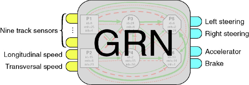
Figure 12.12 The GRN uses nine track sensors and longitudinal and transversal speeds to compute the car steering, acceleration, and brake.
To simplify the problem, the gear value is handwritten as it is a very simple script to develop; when the motor is over a given threshold that depends of the current gear, the driver shifts up. Under another threshold, the driver shifts down.
Figure 12.13 presents how the protein chromosome of the GRN is ordered: the first 11 proteins are input proteins, the next four are output proteins and the remaining ones are regulatory proteins. Whereas the input and the output proteins can be crossed over or mutated, they cannot be deleted.

Figure 12.13 Organization of the protein chromosome and link to the car sensors and actuators: protein tags (in red) are evolved by the genetic algorithm whereas protein types (in green) are fixed and always plugged to the same car sensors (for input proteins) and the same car actuators (for output proteins).
In order to optimize the GRN to drive a car, we use an incremental evolution in three stages.3 During these stages, the same parameters have been used to tune the genetic algorithm. Only the fitness function is modified. The genetic algorithm parameters are
- population size: 500,
- mutation rate: 15%,
- crossover rate: 75%,
- GRN Size: [4, 20] regulatory proteins plus inputs and outputs.
The first stage consists of training the GRN to drive as far as possible, with a minimum speed, on one track. We use CGSpeedway, the left-hand side track provided by the car simulator (see Figure 12.14), which is simple with long turns and straight lines. This track is interesting for learning to drive because it is a relatively simple track with long fast turns and with fast straight lines to learn how to steer and to accelerate, and with more difficult short turns to learn how to slow down and to brake. Each GRN is tested on this track for 31 kilometers (about 10 laps) maximum. The simulation is stopped as soon as the car leaves the track or gets damaged (by hitting a rail for example). To ensure the car is driving fast enough, we use a ticket system in which the GRN must cover 500*nLap meters per 1000 simulation steps, where nLap is the current lap number. This pushes the GRNs that go far to accelerate. If a GRN cannot reach this goal, the simulation is stopped. When the simulation ends, the fitness function is given by the distance covered by the GRN along the central line of the track. If a GRN has traveled all 31 kilometers, a bonus is added. The bonus is inversely proportional to the number of simulation steps needed to complete the race (the faster, the better).

Figure 12.14 Tracks used to train the GRN. All of them are provided by TORCS.
After evolving GRN with a genetic algorithm, we obtain a GRN that is able to drive endlessly on this track. It is a safe driver that regulates its speed so that it can go through all the turns of this track. However, we observed that this GRN is not able to drive on other tracks. In fact, as presented on Figure 12.15, the car is slightly shifted to the right side of the track. That might explain why the GRN cannot generalize its driving: most of the turns on the training track are left-handed. Thus, staying on the right side is better. However, on tracks with hard right turns, this position can be dangerous, the angle for right turns being closed. Moreover, some significant oscillations on the steering can be noticed. Even if they do not imply oscillations on the car track position, this behavior is unwanted and can be harmful in a car race. The aim of the next evolution stages is to correct these defects.

Figure 12.15 Evolution of the car behavior during the three different stages of evolution. The left-hand side plot represents the car position on the track along the distance from the start line: 0 means the car is on the track centerline, −1 means the car is on the right edge of the track and 1 means the car is on the left one. The right-hand side plot is the steering output value along the distance from start. −1 means the steer is fully rotated to the right and 1 means fully rotated to the left.
From these observations, we evolved the GRN to safely cover all possible tracks, with all possible kinds of turns. With this aim in mind, we evolved the previous GRN a second time with the same evolutionary process but on three different tracks. The tracks used are CGSpeedway (in order not to lose the driving capacity of the previous GRN), Alpine and Street, whose layouts are presented in Figure 12.14. The fitness function consists of summing the fitness value defined during the first evolution stage successively applied to the three tracks.
At the end of this evolution, the best GRN is able to drive on every possible track. It drives very safely, going at a suitable speed to go through every kind of turn and braking when it detects a turn. However, the best GRN has an oscillatory behavior and is slightly shifted to the right-hand side of the track. Whereas oscillatory behaviors are common in gene regulatory networks, both these issues could be harmful during a car race. This oscillation can be observed in Figure 12.15 where the trajectories and the steering of the car are plotted during the second lap on one of learning tracks (CGSpeedway). This oscillatory behavior can still be noticed on the steering plot in which the blue curve, which represents the second stage of evolution, strongly oscillates. The result is some parasitic behavior of the car on the trajectory, especially at the end of the turns. The final cleaning stage aims to reduce these parasitic behaviors.
To minimize oscillatory behaviors, we re-optimize the best GRN one last time. This time we add to the fitness function another test case that penalizes continuous oscillations of the car on straight lines and long turns or fast multiple steering changes from full right to full left. As with the ticket system or the damage control used in the previous fitness functions, we simply stop the evaluation if we detect oscillatory behaviors.
The green line on Figure 12.15 shows the steering values of the best GRN on CGSpeedway track at the end of this evolution stage. The steering spikiness of the previous evolution (blue curve) that is visible in the first two fast curves is smoothed and the steering does not oscillate anymore from full right to full left in the track section from turn 4 to turn 8 and from turn 9 to turn 1 (see Figure 12.14).
It can be noted that this last evolution stage reinforces the generalization stage by improving the central position of the car. The GRN is also faster than before because the oscillations slow the car down. These multiple evolution stages were then strongly efficient to produce a GRN able to drive the car efficiently on most of the tracks. Another property emerges from the evolved GRN: it is also able to adapt to various kinds of track surfaces such as rock and sand, with no reoptimization. The GRN is also resistant to sensor noise. This is an uncommon result since most other approaches used to control a car are based on noise reduction systems and, even with these systems, are still impacted by the noise (more details can be found in Ref. [22]). Both adaptativity and noise resistance are crucial properties for agent control since they allows the agent to handle uncertainty in the environment. Moreover, these are necessary to bridge the reality gap when such a system is used in real robots.
12.6 REGULATING BEHAVIORS
In this last example of application of the gene regulatory network, instead of connecting the GRN directly to the agent sensors and actuators, we propose to use the GRN to regulate high-level behaviors in each agent of a team. For this purpose, we have designed a defense/interception mission in which a team of agents has to defend a target and intercept incoming threats. Multiple defending agents have to coordinate their behavior with local information only (e.g., distance to the target to defend, to the next threat, to teammates, etc.) in order to intercept as much as possible threats coming sequentially or simultaneously from random position. The objective of the threats is to destroy the target. Because this study focuses on the defending agent behaviors, the threat behavior has been kept very simple: they are driving to the base at various speeds, following random checkpoints.
The behavioral architecture is based on a three-layer structure: the top layer, named behavior layer, is a set of high-level behaviors that provides specialized functionalities to the agent; the intermediate layer, named control layer, is an aggregation layer, where all decisions taken by the high-level modules are regulated to generate the global behavior of the agent; the bottom layer, named actuation layer, is used to actuate the agent in the environment and to apply the actions generated by the upper layer.
Applied to our defense problem, defending agents have access to four driving behaviors (top layer) which are: defense (drives to the target to defend), interception (drives to the threat), scattering (drive away from defending group gravity center), and grouping (drive to the gravity center). This architecture uses the GRN described in Section 12.2 as behavior aggregator. In this approach, instead of controlling agents at a very low level (e.g., control the wheel rotation speed), the GRN weights each driving behavior by the mean of one output protein per driving behavior.
To generate the driving direction, the GRN regulates the defending, intercepting, grouping, and scattering behaviors by weighting the vectors generated by these behaviors. The final movement ![]() of agent a is given by
of agent a is given by ![]() , where
, where ![]() (resp.
(resp. ![]() ,
, ![]() and
and ![]() ) is the vector provided by the defense (resp. interception, grouping and scattering) behavior. Each weigth wi is calculated with the concentration of four output proteins:
) is the vector provided by the defense (resp. interception, grouping and scattering) behavior. Each weigth wi is calculated with the concentration of four output proteins: ![]() where ci is the concentration of the protein associated with the weight wi. Figure 12.16 depicts the use of a GRN to regulate defending agents’ driving behaviors.
where ci is the concentration of the protein associated with the weight wi. Figure 12.16 depicts the use of a GRN to regulate defending agents’ driving behaviors.

Figure 12.16 Integration of the high-level behaviors and of the GRN to the three-layer behavioral architecture.
To evaluate this approach, we imagine a mission in which the agents have to coordinate their strategies in order to defend a target against a sequence of incoming threats. The threats are incoming sequentially in the environment from random positions. The complexity of the task also increases with the arrival of new threats: the speed of each new threat is increased so that it gets harder to intercept. Therefore, the main aim of this experiment is to coordinate the defender team in order to intercept as many threats as possible and produce global strategies in order to intercept fast threats.
To tackle this problem, the GRN uses the following inputs: a defender–enemy distance morphogen, the defender/threat speed ratio, an enemy–target distance morphogen, an agent–allies distance morphogen, the team interception level (average level of interception of all the defending agents) and the position of the agent in the team according to their distances to the threat. These inputs allow each defender to evaluate their position in the team, their position relatively to the target to defend and to the threats and the dangerousness of the current threat. They provide the concentration of the GRN’s input proteins.
A standard genetic algorithm evolves the GRN. Each individual is evaluated on three random scenarios with a sequence of 100 threats. Threats’ speeds linearly increase from 70% to 120% of defender speeds. The fitness of a GRN is the sum of the fitness obtained on three random scenarios. Each scenario is evaluated by a fitness function that takes into account the lifetime of the threat before interception. This function is designed to promote controllers that intercept threats as far as possible from the target to defend.
The genetic algorithm is run 48 independent times in order to produce diverse team strategies. As presented in Figure 12.17,4 four main strategies emerge:
- the minimal team strategy that builds the minimal team to intercept the threats;
- the line strategy that positions the defenders along a line between the target to defend and the threat;
- the wing strategy that aligns the defenders along an orthogonal line between the threat and the target; and
- the grid strategy that divides the space into sectors and allocate a defender per sector.

Figure 12.17 Strategies that emerge from independent training of the GRN. From left to right, the first one consists in creating a “wing” between the target to defend and the threat. In the second strategy, defenders are distributed on the line between the target and the threat. The third strategy consists of sending one defender at the time to intercept the threat and, if it fails, other defenders are available to be sent in back up. Finally, the last strategy consists of dividing the space into sectors and have one defender in each sector. These sectors are dynamical: they change according to the threat position, dangerousness and direction. This improves the capacity of the defenders to intercept the threats.
We have compared the GRN-based approach to a script provided by defense experts. The script allocates the closest defender to the threat between the target to defend and the threat as an interceptor, driving it to the interception point as fast as possible. The second and third closest, named the wingers, are positioned on both sides of the interceptor at a distance equal to the distance separating the threat and the interception point of the interceptor. These defenders produce a wing-like formation. The fourth defender, called the protector, is positioned between the threat and the target to defend. If the team is composed of more than four defenders, other teammates are kept on the target to defend. If the team is smaller, the wingers are deleted first before the protector. Figure 12.18 compares the results of the GRN-based approach against the scripted one. The comparison consists of 30 random scenarios. A scenario is initialized with 100 threats to intercept with a four-defender team. The threats are randomly positioned in the environment and have a random checkpoint list to follow before colliding on their target. Each scenario is played with various speed ratios (the higher the ratio, the faster the threats in comparison to the defenders) to evaluate the capacity of the approaches to handle simple and complex situations. For both approaches, we provide the maximum (in blue), the minimum (in red), the median (in purple), and the first quartile (in green) of the success rates on the pool of scenarios. Because the problem is to defend a target, the worst-case scenario is the most important measure. With this measure, we can observe that the GRN is doing better than the script: the minimum success rate is kept to 100% with higher speed ratios with the GRN than with the script. Moreover, the first quartile is dropping down with the scripted approach with a speed ratio between 1.05 and 1.10 whereas the GRN approach is able to keep it to 100% for all speed ratios. This means the GRN is better at adapting to faster threats than the scripted approach due to the capacity of the GRN to adapt to unknown situations.

Figure 12.18 Comparison of the best GRN (left-hand side) approach and the scripted approach (right-hand side) on 30 random scenarios composed of 100 threats to intercept with various fixed speed ratios (abscissa). The minimum success rates (worst-case scenario, in red) drops faster with the scripted approach than with the GRN (vertical dashed line): the GRN adapts better to higher speed ratios than the scripted approach.
Another property of the GRN approach is its ability to adapt the strategy to the size of the team with no further learning. Figure 12.19 shows this property on the grid strategies where defenders modify their positions in the environment according to allies positions: the switch from a square to a triangle or a pentagon. Moreover, the structure is twisted according to the threat position. Comparable observations can be made on the wing, the line, and the minimal team strategies. This generalization on the number of defenders is inherent to the system because all the data used by a defender to take its decision (via the GRN) are local and relative. Therefore, defenders can be added or removed from the system without impacting the decision process. This team size adaptation can even be done during the simulation without perturbing the system.

Figure 12.19 Example of system adaptation to the team size: the same GRN is used to handle teams composed of three, four, or five defenders. The team covers the environment according to the team size.
12.7 CONCLUSION
In this chapter, we have presented three applications of a computational model of a gene regulatory network. We showed how to directly connect the network’s inputs and outputs to the agent sensors and actuators in the artificial embryogenesis and the car driving problems. Then, we showed that the GRN can also be used at a higher level, to regulate agent behaviors in a cooperation mission. In all these experiments, crucial properties for virtual agents emerge from the system: the GRN can generate behaviors both resistant to noise and adaptive to unknown environment.
The domain of applications of gene regulatory networks is extremely wide. It can be easily applied to many agent-based problems. Indeed, we showed in this chapter that the GRN is able to generate very complex behaviors. However, the complexity can be double-edged: evolving gene regulatory networks with standard evolutionary algorithms can be difficult. Developing an evolutionary algorithm dedicated to evolve gene regulatory networks might help to handle this complexity, as NEAT was meant to evolve neural networks [23]. Currently, most evolutionary algorithms used to evolve gene regulatory networks are mainly based on mutation and few of them use crossover. Actually, crossover usually induces too many modifications in the network structure to be efficient. Therefore, finding a crossover that conserves the global structure of the network would improve the convergence of the evolutionary algorithm. As used in NEAT, historical markers that identify key genes, present in the network for a long time, could be a first line of research since similar mechanisms exist in nature. That could help the GRN to address more complex problems making it capable of exploiting more inputs to regulate more outputs.
NOTES
REFERENCES
- Torcs: The open source racing car simulator. http://torcs.sourceforge.net
- W. Banzhaf. Artificial regulatory networks and genetic programming. In R. L. Riolo and B. Worzel, editors, Genetic Programming Theory and Practice. Springer, Chapter 4, pages 43–62, 2003.
- A. Chavoya and Y. Duthen. A cell pattern generation model based on an extended artificial regulatory network. BioSystems, 1–2:95–101, 2008.
- S. Cussat-Blanc, N. Bredeche, H. Luga, Y. Duthen, and M. Schoenauer. Artificial gene regulatory networks and spatial computation: a case study. In Proceedings of the European Conference on Artificial Life (ECAL’11). MIT Press, Cambridge, MA, 2011.
- S. Cussat-Blanc and J. Pollack. A cell-based developmental model to generate robot morphologies. In Proceedings of the 14th Annual Conference on Genetic and Evolutionary Computation. ACM New York, NY, 2012.
- S. Cussat-Blanc and J. Pollack. Using pictures to visualize the complexity of gene regulatory networks. In Artificial Life, volume 13. MIT Press, pages 491–498, 2012.
- S. Cussat-Blanc, S. Sanchez, and Y. Duthen. Simultaneous cooperative and conflicting behaviors handled by a gene regulatory network. In 2012 IEEE Congress on Evolutionary Computation (CEC), pages 1–8. IEEE, 2012.
- H. de Garis. Artificial embryology and cellular differentiation. In Peter J. Bentley, editor, Evolutionary Design by Computers. Morgan Kaufmann, pages 281–295, 1999.
- F. Dellaert and R. Beer. Toward an evolvable model of development for autonomous agent synthesis. In Artificial Life IV, Cambridge, MA, 1994. MIT press.
- J. Disset, S. Cussat-Blanc, and Y. Duthen. Self-organization of symbiotic multicellular structures. In ALIFE 14: The Fourteenth Conference on the Synthesis and Simulation of Living Systems, volume 14. MIT Press, pages 3–5.
- R. Doursat. Organically grown architectures: creating decentralized, autonomous systems by embryomorphic engineering. Organic Computing. Springer, pages 167–200, 2008.
- P. Eggenberger Hotz. Combining developmental processes and their physics in an artificial evolutionary system to evolve shapes. On Growth, Form and Computers. Academic Press, page 302, 2003.
- N. Flann, J. Hu, M. Bansal, V. Patel, and G. Podgorski. Biological development of cell patterns: characterizing the space of cell chemistry genetic regulatory networks. Lecture Notes in Computer Science, 3630:57, 2005.
- M. Gardner. The fantastic combinations of John Conway’s new solitaire game life. Scientific American, 223:120–123, 1970.
- Hongliang Guo, Yan Meng, and Yaochu Jin. A cellular mechanism for multi-robot construction via evolutionary multi-objective optimization of a gene regulatory network. BioSystems, 98(3):193–203, 2009.
- M. Joachimczak and B. Wróbel. Evolving gene regulatory networks for real time control of foraging behaviours. In Proceedings of the 12th International Conference on Artificial Life. MIT Press, 2010.
- M. Joachimczak and B. Wróbel. Evolution of the morphology and patterning of artificial embryos: scaling the tricolour problem to the third dimension. In Advances in Artificial Life. Darwin Meets von Neumann, pages 35–43. Springer, 2011.
- J. Knabe, M. Schilstra, and C.L. Nehaniv. Evolution and morphogenesis of differentiated multicellular organisms: autonomously generated diffusion gradients for positional information. Artificial Life XI, 11:321, 2008.
- R.P. Lifton, M.L. Goldberg, R.W. Karp, and D.S. Hogness. The organization of the histone genes in drosophila melanogaster: functional and evolutionary implications. In Cold Spring Harbor Symposia on Quantitative Biology, volume 42, pages 1047–1051. Cold Spring Harbor Laboratory Press, 1978.
- M. Nicolau, M. Schoenauer, and W. Banzhaf. Evolving genes to balance a pole. In A. I. Esparcia-Alcazar, A. Ekart, S. Silva, S. Dignum, and A. Sima Uyar, editors, Proceedings of the 13th European Conference on Genetic Programming, EuroGP 2010, volume 6021 of LNCS. LNCS, pages 196–207, 2010.
- T. Reil. Dynamics of gene expression in an artificial genome-implications for biological and artificial ontogeny. Lecture Notes in Computer Science, 457–466, 1999.
- S. Sanchez and S. Cussat-Blanc. Gene regulated car driving: using a gene regulatory network to drive a virtual car. Genetic Programming and Evolvable Machines, 15(4):477–511, 2014.
- K. O. Stanley and R. Miikkulainen. Evolving Neural Networks through Augmenting Topologies. Evolutionary Computation, 10(2):99–127, 2002.
- J. Von Neumann and A.W. Burks. Theory of Self-reproducing Automata. University of Illinois Press, 1966.
- L. Wolpert. Positional information and the spatial pattern of cellular differentiation. Journal of Theoretical Biology, 25(1):1, 1969.