
CHAPTER 14
REGULATORY REPRESENTATIONS IN ARCHITECTURAL DESIGN
Daniel Richards and Martyn Amos
School of Computing, Mathematics and Digital Technology, Manchester Metropolitan University, Manchester, United Kingdom
14.1 INTRODUCTION
In this chapter, we consider the application of evolutionary algorithms and regulatory networks to problems in architectural design. The “cybernetic theory of architecture” dates back to 1969, when Pask [49] predicted that “Various computer-assisted (or even computer-directed) design procedures will be developed into useful instruments” for the design of buildings and cities. Pask’s ideas about control and communication were developed by architects such as John Frazer, who were interested in how concepts of adaptation might be applied to the design, construction and evolution of building form and performance. In An Evolutionary Architecture, Frazer sets out how natural processes might be harnessed as “the generating force for architectural form” [19]. Importantly, he seeks to go beyond the rigid and specific “blueprint” metaphor, and to develop a “genetic language of architecture”, in which form-generating processes give rise to structure and behavior. Since then, evolutionary design in architecture has become well-established [6, 7, 16]. However, many such syntheses have still been modelled on what Oxman [48] calls the cyclical “generate and test” paradigm, in which conceptual design generation is followed by performance evaluation. Oxman argues that this approach naturally follows from the traditional way in which architectural designs have been conceived, designed and built, where form takes priority over performance. The “form-first” approach, in which “real world” performance (such as structural integrity or temperature regulation) is considered relatively late, can lead to designs that are wasteful in terms of material, are much less integrated, and are inherently less sustainable. An alternative performative [48, 66] paradigm seeks to invert this approach, so that “features such as material properties, fabrication constraints and environmental performance are allowed to influence the early development and synthesis of form” [55]. In order for such an approach to be successful, we require new forms of representation for computational design synthesis, and in this chapter, we discuss recent developments in this area. We describe previous foundational work, and motivate and support the need for such representations, before describing our developmental mapping process. We then investigate specific properties of our “evo-devo” model, which, we argue, allows us to exploit neutral mutations and thus produce evolutionary innovation. We present extensive experimental results to support our claim before concluding with a discussion and suggestions for future work.
14.2 BACKGROUND
Computer technologies have transformed architectural design. The proliferation of computer-aided design (CAD) software has significantly enhanced the control and analysis of three-dimensional designs [5], while computer-aided manufacturing (CAM) has created entirely new opportunities for large-scale construction [23]. CAD/CAM technologies provide designers with new abilities to design and construct complicated three-dimensional geometries. However, an important open question for design research is: can these technologies do more? Principally, can advanced computational design techniques facilitate new forms of architecture that are highly efficient and increasingly performance-oriented?
Within architectural design, a key motivation is “sustainability.” That is, to address issues such as climate change and rapid urbanization, architects and engineers require new methods of designing built forms that minimize or mitigate environmental impact [65]. There exists much current debate over what constitutes a “sustainable” solution [41], but the basic argument is that designers should use CAD/CAM technologies to do more with less. This means that architects should seek to design performance-driven structures that are more efficient and more multifunctional, while also being less energy intensive and less wasteful in their use of material resources. The problem, however, is that designing complex multifunctional structures is significantly challenging. To address this, recent work has advocated the application of bio-inspired approaches to design that aim to simulate natural processes of formation in order to generate efficient material-based structures [37, 47].
Biological structures have extraordinary physical properties, and have inspired designers and engineers for generations [18]. However, biological structures are not designed; rather, they emerge through a synthesis of complex natural processes. That is, by combining Darwinian evolution with complex and stochastic physical or developmental processes, nature assembles extremely efficient material structures that are economical, multifunctional and often (to human eyes) beautiful. These structures may be much more complex than anything we can currently design (we are currently nowhere near synthesizing even the simplest microbe), but the ability to harness the underlying processes for computation would provide significant advances in the field of architectural design.
The idea of using bio-inspired algorithms to generate useful architectural structures within computers (or “in silico”) represents a growing area of interest [26, 60, 76]. So far, however, existing work remains either entirely theoretical, or describes bio-inspired analogies that relate to semi-automated design processes. The critical question for this emerging area of research is: what type of computation is required to synthesize complex and multifunctional material structures? In the context of this chapter, the term “computation” refers to a process of transforming a series of inputs (such as material properties, structural performance or fabrication constraints) into three-dimensional outputs. Hence the question could be restated as: what types of algorithmic processes (digital or analogue) are required to transform a set of known constraints and physical properties into complex and multifunctional architectural forms? Once we address this, we then naturally seek to understand how these processes facilitate the evolution of form. In what follows, we present investigations into both questions.
14.3 THE NEED FOR REGULATORY REPRESENTATIONS
Biological organisms are complex adaptive systems that demonstrate two remarkable, yet seemingly opposing characteristics. First, biological organisms demonstrate the extraordinary capacity to innovate and evolve novel phenotypic traits to exploit specific environmental niches. Second, biological organisms are robust to a great deal of genetic and environmental perturbations, showing a profound ability to persist when conditions change or parts fail. A key challenge for evolutionary computation (and associated engineering domains) is to consider which principles of biological systems can be extracted and used to build similarly efficient artificial systems [33, 63]. Indeed, the question of how to exploit self-organizing processes in order to build efficient artificial systems is arguably the “meta-problem of engineering” [36]. Critically, for many engineering domains, an ideal evolutionary system would be robust enough to allow fine-grained optimization of well-constrained phenotypic attributes; but it would also be flexible enough to explore a diverse set of solutions when prior information about the design problem is unavailable [2]. That is, an ideal system would (perhaps paradoxically) be robust and well constrained, yet flexible and capable of radical innovation. However, constructing encodings (genotypes) and representations (genotype–phenotype mappings) that facilitate both types of opposing properties is a challenging problem [12, 63]. Typically, representations tend to be either: (1) highly constrained (i.e., rigid), enabling efficient parameter optimization [30]; or (2) highly flexible, yet brittle, enabling “creative” exploration of diverse solutions that may, or may not, be buildable in the real world [8, 45, 46]. As Roudavski explains [60], a design space is defined by (and thus restricted to) the set of variables that are accessible to a designer, and “unconventional, lateral, associative moves are often necessary to expand this space and to find in it innovative outcomes.”
We have previously argued [53, 54, 55] that evolutionary design systems, which simultaneously invent and calibrate well-constrained variables, will lead to next-generation CAD software and facilitate game-changing opportunities in numerous engineering domains. Consequently, our ongoing research has sought to bridge this gap between “highly constrained” and “highly flexible” representations in order to facilitate the evolution of diverse three-dimensional morphologies for real-world problem domains. We have previously presented a novel representation inspired by gene regulatory networks and used it to evolve three-dimensional structures for architectural design [55]. In this work, our evolved structures address multiple real-world performance objectives (such as structural efficiency and capacity to provide solar shading), while the material properties and size of elements were constrained to the machining limitations of specific digital fabrication equipment (Figure 14.1). Our findings demonstrated that our gene regulatory network-inspired representation could generate functional three-dimensional structures in response to a simple multi-objective design problem, and—critically—that the evolved structures had performance qualities comparable to those of a similar human designed solution. That is, the evolved solutions obtained similar levels of structural efficiency (i.e., ability to resist deflection under loading) and solar performance (ability provide a specific uniform level of shading over a period of time), yet often used much less material, and were therefore more cost-effective. However, the significance of this proof-of-principle study was not the direct performance comparison between the human-designed solutions and evolved designs, but that our gene network representation could discover and then optimize functional three-dimensional characteristics without explicit parameterization. For example, the arch-like characteristics of evolved designs (as shown in Figure 14.1) were not explicitly parameterized but emerged from evolved interactions within our gene networks.
We believe that this work represents an important first step toward next-generation CAD tools. Specifically, we think the model holds important clues for creating sophisticated indirect representations that can solve truly complex design problems by eliminating reliance on highly- constrained direct representations that are known to be limited as problems increase in scale and complexity [63, 67].
By examining the evolutionary dynamics of our model, this chapter demonstrates how our regulatory representation can facilitate the desirable, yet seemingly opposed properties of being highly constrained and able to innovate. First, we describe our encoding and developmental representation. Second, we describe our testable hypothesis that our model exploits redundancy and neutrality within robust canalized genomes to facilitate enhanced evolutionary innovations. Third, we present our analysis and results, and finally, we conclude with a discussion of ongoing challenges and exciting opportunities for further work.

Figure 14.1 (a) Evolved canopy, (b) structural analysis, and (c) solar analysis. Reprinted with permission from Ref. [55], copyright 2012 Association for Computing Machinery, Inc.
14.4 DEVELOPMENTAL MAPPING
Our model controls how a fixed number of nodes interact within a volume to create buildable three-dimensional structures (Figure 14.2). The encoding is a simple fixed string genome and the representation, which takes inspiration from gene regulatory networks, works by sequentially activating each node’s associated growth instructions to construct three-dimensional designs that can then be subjected to various performance evaluations (such as structural analysis).

Figure 14.2 Model setup. A three-dimensional volume contains a fixed number of node objects. These nodes are encoded with simple growth instructions, which are used during the developmental representation to grow three-dimensional designs. Reprinted with permission from Ref. [55], copyright 2012 Association for Computing Machinery, Inc.
14.4.1 Encoding
Each node is described by a 10-digit gene, which can be broken down into four gene attributes (Figure 14.3a). These four gene attributes define four aspects of how nodes grow local connections and ultimately assemble larger network structures. First, each node has a “range of influence,” ROI, which defines a radial dimension (or neighborhood) within which it can communicate with other nodes (Figure 14.3b). Second, each node has an explicit Cartesian position, XYZ, within the three-dimensional volume (Figure 14.3c). Third, nodes are able to make different geometric connections, G, between their neighboring nodes (i.e., within their ROI). In our initial experiment, we limited these different geometries to simple struts between neighboring nodes (Figure 14.3d), closed rings (Figure 14.3e) and “petal”-shaped components (Figure 14.3f). Finally, nodes can create connections that have various material properties, M, and/or different size cross-sectional areas. As shown in Figure 14.2, our model also has explicitly defined anchor points (denoted by the cubes), these points are necessary when performing structural analysis calculations, and simply provide fixed supports that nodes can connect with in order to distribute loads to the ground plane (see Ref. [55] for full details).

Figure 14.3 Genotype structure: (a) Each node is described by four genes, which define four aspects of its development: ROI, M, G, and [X, Y, Z]. (b) The range of influence (ROI), a radial dimension, described by a two-digit gene (in the range 0–99), within which nodes can perceive, communicate, and connect to other nodes. (c) The position of the node within 3D space as described by a six-digit gene (each digit in the range 0–9) that defines the Cartesian coordinates [XX, YY, ZZ]. (d–g) The library of geometry types, G, which the node uses to construct structural connections within its ROI. This is specified using a one-digit gene (in the range 0–9) to select either: G1, G2, or G3. Reprinted with permission from Ref. [55], copyright 2012 Association for Computing Machinery, Inc.
14.4.2 Representation
The developmental mapping activates the growth instructions of all individual nodes to assemble a larger three-dimensional structure. During this process, each node operates as a spatially embedded genetic switch that, when activated, constructs various types of geometric, G, and material, M, connections between nodes within its ROI. However, grown network structures represent physical three-dimensional designs and, consequently, the connections have a structural depth as well as two key fabrication and assembly constraints that need to be respected. First, there can only ever be one connection between any two nodes (to prevent intersecting geometry) and second, depending on the fabrication method, connections must also not intersect while crossing in three-dimensional space.
To enforce these physical constraints, we sequentially activate nodes, using a fixed order of activation defined by node index. This means that the order in which nodes construct connections is significant. Critically, nodes that are activated early in the growth process indirectly modify the growth of subsequent connections via the process of positive and negative regulation. Positive and negative regulation is observed in biological processes of gene expression [75]. Put simply, genes are switched “on” or “off” by the existence, or non-existence, of specific proteins (in reality, genes are rarely binary). If a gene is switched “on,” or expressed, a protein is produced, which, in turn, will control the expression or repression of further genes through positive regulation. Conversely, if the gene is switched “off,” or repressed, no protein is transcribed, which influences the expression or repression of further genes by, what is termed, negative regulation. While existing works use biologically analogous models of gene regulation to evolve complex morphologies [14, 4], our model makes no such attempt to accurately model gene regulatory networks. However, we do utilize the basic mechanism of positive and negative regulation to produce three-dimensional structures that are described by complex regulatory dependencies.
To ensure that there is only ever one connection between any two nodes, each node is given a small “memory space” which stores information about all other nodes to which it is currently connected. Before a node creates a connection with another node (i.e., within its ROI defined neighborhood), it first checks that it does not already have an imprint of that node (analogous to a protein) in its memory space (analogous to a cis-regulatory region of DNA). If the node finds an imprint, then no connection is made, but if no imprint is found then a new connection is made and each node exchanges a copy of their unique imprint to prevent further connections being made. To illustrate this process, Figure 14.4 describes the developmental growth and imprint change system in more detail. For clarity, the nodes are set on a two-dimensional plane and each node is defined using only three gene attributes: ROI, M, G. Each node’s memory space is shown as square brackets that hold the node index value (imprint) of nodes that they are connected to. Notably, Figure 14.5 illustrates that small changes to gene attributes can cause significant alterations to the phenotypes through positive and negative regulation.

Figure 14.4 Developmental growth. (a) Shows a random arrangement of nodes with empty memory spaces. (b) Node 1 grows G1 connections between itself and nodes within its ROI. (c) Node 2 grows G2 connections between surrounding nodes omitting Node 1 as it already has a connection. (d) Nodes 3 and 4 have been repressed by Node 2’s earlier growth. Reprinted with permission from Ref. [55], copyright 2012 Association for Computing Machinery, Inc.

Figure 14.5 Phenotype variability. Small changes to node ROI or geometry type can dramatically influence phenotype formation through positive and negative regulation. (a) Phenotype produced from Figure 14.4. (b) Mutation of Node 1 geometry type|G1 to G2. (c) Mutation of Node 2 geometry type|G2 to G1. (d) Mutation of Node 2 ROI - ROI = 7 to ROI = 2. Reprinted with permission from Ref. [55], copyright 2012 Association for Computing Machinery, Inc.
To address the second physical constraint and ensure buildable phenotypes, we perform a maximum of two further processes to prune unbuildable connections. First, if physical connections are fabricated using a discrete assembly of parts, such as steel struts, we prune connections that intersect within three-dimensional space (Figure 14.6a). Note that this process may not be necessary when using certain fabrication methods such as additive manufacturing (i.e., 3D printing). Second, disconnected parts of the structure that are not supported within space (i.e., floating parts) are removed (Figure 14.6b). Critically, following the sequential activation of growth instructions and potential pruning steps, phenotypes are always buildable and suitably constrained for physical assembly and digital simulation processes.

Figure 14.6 Pruning process. (a) Following the developmental growth process, if any components intersect the last component to be formed is deleted. (b) Following the intersection test, a connectivity test is used to identify and remove any components that are disconnected from the main structure. Reprinted with permission from Ref. [55], copyright 2012 Association for Computing Machinery, Inc.
14.4.3 Experimental Results
To test the evo-devo representation, we set it the task of designing an economical, free-standing structure that can provide controlled (passive) solar shading of a space during the summer months, and may be fully fabricated using 1 mm CNC cut aluminium sheets. For brevity, full details of the experiments are supplied in Refs. [54, 55], and the results are shown in Figure 14.1.
Briefly, the fitness of each phenotype is calculated using the weighted sum of four performance measures: first, the average nodal deflection of structures under loading was considered. Second, a measure of the average height of structural nodes was used. Third, total fabrication cost was considered, based on material usage, and finally, a measure of daily solar performance was used. Structural fitness (StF) is calculated using physical simulation. The average combined deflection in [x, y, z] position of structural nodes (AvD) is compared with an acceptable nodal deflection value (AcD) and an unacceptable deflection value (UaD) that defines the breaking point of the component when subjected to a combination of dead weight of structure and an imposed 0.2 kN wind loading:

Height fitness (HeF) is defined by the average height of structural nodes (AvH) in relation to the maximum build volume height (BvH). In this experiment, tall models are favored in an attempt to consider how accommodation requirements of structures might be evolved in larger models:
The total fabrication cost (CoF) is defined by the required amount of aluminium sheeting (ReA) to fabricate the structure. This is compared against a defined fabrication budget (FaB) and a maximum overspend allowance (MoS). For illustrative purposes the FaB = £300 and MoS = £500.

Solar fitness (SoF) is defined by the average difference (AvDiff) between each solar analysis grid cell and a desired measure of solar performance (DeS). Full exposure of any grid cell during analysis returns 2400 kWh. For illustrative purposes, DeS = 1500 kWh.

Finally, the overall fitness of each phenotype (F) is calculated by the weighted sum of StF, HeF, CoF, and SoF. The relative weightings correspond to the importance of each performance-based attribute in the architectural solution
where w1 = 1.5, w2 = 1, w3 = 0.5.
The genetic algorithm (GA) parameter settings used in this section are shown below:
| Population size | 100 |
| Generations | 60 |
| Independent runs | 10 |
| Selection type | Tournament |
| Tournament size | 5 |
| Crossover type | One-point |
| Crossover rate | 100% |
| Mutation rate (per gene) | 0.005% |
14.5 ROBUSTNESS AND EVOLUTIONARY ADAPTATION IN BIOLOGICAL SYSTEMS
The link between robustness and evolutionary innovations within biological systems is not well understood and represents an ongoing area of investigation with many open questions [1, 22, 34, 42, 74]. Various works demonstrate that biological systems are often extremely robust to genotypic and environmental perturbation [61]. Indeed, phenotypes often seem protected, or buffered, against a large amount of internal (genetic) and external (environmental) variations. This mutational buffering is termed “canalization” [70]. As noted by Stanley and Miikkulainen [63][p. 113], Waddington’s use of the term canalization draws an analogy between “the way water running down a hill eventually carves out regular streams in the surface, and the way development slowly settles on a set of conventions that become ingrained in the genome.” Critically, this means that a canalized genome is less sensitive to certain perturbations and thus more likely to produce consistent phenotypic traits. The origins of mutational robustness and canalization remain the subject of investigation [1, 17, 62, 68]. Yet, existing work suggests they can originate from adaptive evolution [71], or be an emergent property of gene regulatory networks [29]. Canalization is clearly an important property of biological structures because it preserves important phenotypic traits in response to (genetic and environmental) variation and perturbation. Consequently, Stanley and Miikkulainen [63] suggest that biologically analogous mechanisms of canalizing “brittle” (yet flexible) artificial encodings may benefit evolutionary algorithms by providing a safer search through genotypic space. Critically, this ability to optimize highly flexible representations and address real-world problems is a key goal for next- generation CAD tools; therefore, models that can exploit bio-inspired processes and enhance mutational robustness may significantly benefit future design software.
Interestingly, existing work shows that mutational robustness may provide another desirable property and may actively facilitate evolutionary innovations [32, 73]. In the late 1960’s, Kimura [31] proposed that during evolution, many mutations that occur at the molecular level are “silent” or neutral (i.e., do not affect phenotype fitness) and consequently, these mutations are selectively propagated throughout populations via the random process of genetic drift. More recently, research has suggested that these neutral mutations could be the source of innovation and beneficial evolutionary adaptations in biological organisms [13, 15, 74]. Put simply, this means that over generational time canalization allows organisms to accumulate hidden genetic variation [35], which may eventually become non-neutral and facilitate useful evolutionary adaptation [25, 73]. This leads to an interesting question of whether certain types of genome are more likely to acquire novel functionality through genetic change. Put simply, does the ability to evolve itself evolve? From a CAD perspective, this idea is extremely exciting, because representations that could manipulate their sensitivity to mutations might have the capacity to perform both: flexible, explorative search and fine grained optimization of robust three-dimensional parts. The term evolvability is often used to discuss how well an organism can adapt to changing conditions and produce evolutionary innovations; however, we note that the term does not have a generally agreed definition or common methods for measurement [50, 52]. Indeed, computational studies have shown that artificial gene regulatory networks may possess useful properties relating to “evolvability” [1, 10], while further work has also shown that gene regulatory networks may increase mutational robustness simply as a by-product of “developmental stability” [62]. Interestingly, existing work has also explored possible connections between the properties of evolvability, redundancy, and neutrality in evolution. However, this topic remains a contentious topic, with experimental results finding both positive [77] and negative [9] effects of encouraging neutrality and redundancy during evolution search [21, 28].
14.5.1 Hypothesis
Following on from our previous work [55], we developed the working hypothesis that our gene networks become more robust following evolution, and that this increased robustness enables genomes to exploit phenotypically neutral mutations and produce better evolutionary innovations. We now briefly outline two observations from our previous investigations that led us to this hypothesis. First, we observed that mutations to random gene networks seemed to cause more damage (as assessed visually) to the resulting phenotypes than evolved networks. We speculated that this phenotype variability could be associated with disconnected elements in the gene networks (Figure 14.7a) and chaotic cascades of gene expression. That is, because network connections are grown using relative information, rather than relying on explicitly encoded index values in the genomes, the developmental process used to build the gene networks may be fragile and susceptible to disruption. Subsequently, we hypothesized that an evolutionary trait that actively reduces this susceptibility for disruption (thus increasing mutational robustness) may emerge “for free” in our system. This means that our gene networks may develop methods of “buffering” against deleterious mutations (which destabilize, or disrupt the developmental growth of connections) by compensating for certain perturbations using evolved regulatory logics. This idea is consistent with the work of Siegal and Bergman [62], who found that evolutionary selection of developmental stability is enough to evolve mutational robustness in computational gene regulatory networks. Additionally, our regulatory network model shares several similarities with Julian Miller’s Cartesian Genetic Programming (CGP) model [40], which, interestingly, has been used to evolve robust cellular models that can self-repair after perturbation [39]. Indeed, we suggest that Miller’s self-repairing behavior may be the result of a similar need for developmental stability during a growth phase, which would further support our hypothesis that the model may indirectly evolve this form of mutational robustness.

Figure 14.7 Growth and differentiation of gene regulatory networks in two-dimensions. Networks begin with small disconnected connections (a–b) and through evolution become larger functional structures (c–d). Nodes are positioned using Blondel et al.’s [3] method in Python using Thomas Aynaud’s “community” module for NetworkX. Nodes are then sized according to their eigenvector centrality.
Second, we speculated that our evolved genomes might contain a high degree of neutrality and redundancy. That is, due to mutual inhibition of genes during the growth of the gene networks, evolved genomes may have a significant number of redundant genes, which are completely silent and have no phenotypic effect. To test this idea, we replaced our standard genetic algorithm with a simpler (1+9) evolutionary strategy (as favored by Miller’s CGP approach [40]), and found that this considerably improved our search performance. Critically, we hypothesized that this change may produce better evolutionary adaptations by allowing our gene networks to accumulate hidden genetic variation, through the random process of genetic drift, and exploit this neutral “tinkering” via changes to highly connected hub genes. Notably, this idea is consistent with Vassilev and Miller’s findings, which show that neutral mutations improve the evolution of digital circuits when using a CGP approach [69]. Additionally, the idea that biological systems exploit hidden genetic variation to facilitate evolutionary innovations has been widely advocated in recent research [13, 15, 25, 73, 74].
The following section interrogates two key features of our model to explore the role of mutational robustness and evolvability. For clarity, the two features that we expect to play important roles in the evolutionary dynamics of our model are the sequential activation of nodes and pruning of unbuildable connections. First, recall that our encoding does not define specific connections between genes (i.e., no indexed targeting of nodes), but rather specifies a relative connective potential based on four attributes of the gene and a sequential growth process. The significant implication of this sequential growth process is that earlier activation of genes (to grow network connections) can influence the later formation of connections through a primitive form of regulation. Second, the three-dimensional structures described by gene networks are not guaranteed to be build-able. This means that gene networks, as shown in Figure 14.8(b), simply represent an “unzipped” version of the string genome. In order to translate the gene network into a viable three-dimensional phenotype with specific material dimensions and assembly tolerances, we use a secondary pruning process, whereby unbuildable elements are removed, in a similar manner to Nolfi and Parisi’s [44] rationalization of “grown neural networks” (Figure 14.8).

Figure 14.8 Genotype–phenotype mapping process. (a) The genotype is a fixed string genome where all characters are integers between 0 and 9. (b) Directed three-dimensional network of regulated connections between genes–here shown in two-dimensions. (c) Network connections that are unbuildable are removed–shown as red dotted lines. (d) The phenotype represents all buildable three-dimensional connections of the regulated gene network–here shown in two-dimensions for clarity.
14.5.2 Experimental Results
To test our hypothesis, we investigate three properties of the model. First, we show that evolved solutions are more robust to mutations than random gene networks. Second, we show that neutral mutations improve evolutionary search and allow us to generate better three-dimensional designs. Third, we demonstrate how hidden genetic variation facilitates better evolutionary innovations within our gene networks.
The experimental set-up is the same as that described in Section 14.4.3, with the following parameters:
| Population size | 10 |
| Generations | 600 |
| Independent runs | 20 |
| Selection type | Elitism |
| Crossover type | None |
| Mutation rate (per gene) | 0.02% |
14.5.3 Canalization of Gene Networks
We first consider mutational robustness and developmental stability by measuring how well solutions are able to retain phenotypic traits following genetic perturbation. To do this, changes in “locality” are considered. Locality is a measure of how neighboring genotypes correspond to neighboring phenotypes [59]. When small changes to genotypes correspond to small changes in phenotypes, the genotype-phenotype mapping is said to have high locality. Conversely, if small changes to genotypes represent large jumps across phenotype space, the mapping can be considered more volatile and is described as having low locality. High locality has shown to improve evolutionary search [58], but it is also an indicator that solutions are more robust to mutations because they are better able to retain phenotypic traits following genetic perturbation. To establish the similarity between individuals, a measure of phenotypic distance, pDist, is used, which captures the semantic difference between two solutions:
where SizeA is the total connections in phenotype A, CommAB is the number of common connections between phenotype A and B, and DiffAB is the number of different connections between phenotype A and B. Additionally, if (CommAB − DiffAB) ![]() 0 then pDist(A, B) = 1. Note that we use fixed string genomes for all individuals, therefore, SizeA is a constant, and the distance between all solutions is symmetric.
0 then pDist(A, B) = 1. Note that we use fixed string genomes for all individuals, therefore, SizeA is a constant, and the distance between all solutions is symmetric.
To understand how individuals respond to genetic perturbation, we use Raidl and Gottlieb’s [51] measure of mutation innovation, MI, to calculate how much “innovation” (or difference) is introduced into the solution by perturbing genotype
where Xm is the result of perturbing gene, m, in solution X. Thus, MI represents the semantic difference between solution X and the perturbed solution Xm. Notably, MI is directly related to locality [51].
To understand the relative influence of gene m in phenotype X, it is necessary to consider each fixed string genotype (Figure 14.8a) as its associated gene network (Figure 14.8b). That is, to appreciate which changes to genes represent small or large genotypic adaptions, it is important to consider the architecture of the gene networks. To do this, the importance of genes can be measured using their eigenvector centrality. Note the influence of any node within a simple network can be measured by how many incoming and outgoing connections it has, where this number is called the degree centrality. However, a measure of eigenvector centrality takes into account the fact that all nodes are not equal. Consequently, nodes are not measured simply by their number of connections, but also by the influence or “quality” of the nodes with which they share connections [43]. We calculate the eigenvector centrality of nodes using the NetworkX package for Python.
To test robustness of solutions in response to genetic perturbation, we perform gene knockout tests on random and evolved solutions and measure the correlation between MI and eigenvector centrality of the removed gene. Figure 14.9(a) illustrates the MI obtained by removing each gene from 20 random solutions. Figure 14.9(b) then demonstrates the MI obtained by removing each gene, m, in 20 evolved solutions. These results show that random solutions are (1) extremely brittle and (2) contain many redundant genes. This is evidenced in Figure 14.9(a), whereby removal of genes that have fewer important connections (i.e., low eigenvector centrality) can lead to completely different phenotypes (i.e., MI = 1). Conversely, genes that appear to have many influential connections (i.e., high eigenvector centrality) may lead to unbuildable parts of the phenotype (that will be pruned during the developmental mapping); therefore, the elimination of these genes can have zero phenotypic effect (i.e., MI = 0). This behavior indicates that random solutions have unstable developmental processes, which can be easily disrupted by genetic perturbation. However, as shown in Figure 14.9(b), evolved solutions appear to increase locality and thereby increase mutational robustness in response to genetic perturbation. Indeed, here we see an emerging correlation between eigenvector centrality and MI. This means that perturbation of influential genes tends to produce larger phenotypic changes, and conversely, perturbation of less influential genes tend to produce smaller phenotypic effects. Figure 14.9(c) illustrates that evolved solutions are better able to retain phenotypic traits following genetic perturbation and have increased developmental stability and mutational robustness.

Figure 14.9 Changes in locality and mutational robustness. (a) Low locality in random solutions. No correlation between mutation innovation and eigenvector centrality of genes in random solutions. (b) Increased locality in evolved solutions. Correlation between mutation innovation and eigenvector centrality in evolved solutions. (c) Increased mutational robustness in evolved solutions. Cumulative mutation innovation in both random and evolved solutions.
To understand how the genomes of evolved solutions create phenotypes that are more robust to genetic perturbation we plot how individual genes modify their eigenvector centrality over a typical evolutionary run (Figure 14.10). Here we see that following a short period of fluctuation (around 50–80 generations), the gene network appears to become canalized. Significantly, we see the emergence of “hub genes” that have high eigenvector centrality and seem to preserve phenotypic traits by buffering against large and potentially deleterious mutations. We think that this type of mutation buffering or “heuristic bias” [51] emerges simply as a by-product of requiring developmental stability to optimize gene networks, and notably, supports the earlier findings of Siegal and Bergman [62].

Figure 14.10 Typical canalization of a genome. Canalization typically occurs within 100–150 generations and produces noticeable hubs in the gene network. Canalized genomes are better able to retain phenotypic traits following gene knockouts.
The significance of this finding is that gene networks can indirectly control how mutations affect phenotypes and this may make them easier to optimize. Critically, by increasingly the locality of the genotype-phenotype mapping, evolved solutions establish a higher correlation between small changes in gene networks and small changes in phenotypes. Higher locality in traditional bit-string encodings is known to improve evolutionary search [58, 59]. However, it is less well known how locality affects “tree” or network-based encodings in methods such as genetic programming (GP). In GP, previous strategies of improving search have focused on varying mutation rates in order to mediate between explorative search (high mutation rate when fitness is low) and optimization (low mutation rate when fitness is high) [20]. However, through canalization of the gene networks, our approach seems capable of implicitly controlling the effect of mutations on phenotypes, without explicit variations to mutation rates or operators.
14.5.4 Neutral Shaping of Canalized Gene Networks
This section demonstrates that our gene networks perform better evolutionary search when they are able to accumulate hidden genetic variation via neutral mutations and random genetic drift. To show this we compare two sets of results by running the model on the same problem (as detailed in Ref. [55]), with and without neutral mutations, for 20 independent runs. For the purposes of this analysis, it is sufficient to know that our objective function favored tall and structurally stable designs.
The first treatment, which does allow neutral mutations to occur (and thus enable the accumulation of hidden genetic variation via genetic drift), follows Miller’s [39, 40] CGP approach, using a simple (1+9) evolutionary strategy that has one significant feature. That is, during selection, if two or more phenotypes obtain an equally good fitness score, the phenotype selected to seed the next generation is not the current best. Put simply, the phenotype selected will be “equally fit, but genetically different” from the phenotype selected in the previous generation [38]. In contrast, the second treatment, which does not allow neutral mutations, uses the same evolutionary strategy but only selects phenotypes that are not the current best if they increase fitness. Figure 14.11(a) shows that over 20 test runs, the gene networks that allow neutral mutations perform better. Significantly, genetic drift produces better solutions in around half the time. Figure 14.11(b) illustrates that the model that enables neutral mutations does in fact accumulate hidden genetic variation over time. This is shown by plotting the Hamming distance between consecutive genotypes that increase phenotype fitness throughout evolutionary runs. This plot illustrates, as do Vassilev and Miller’s findings [69], that Hamming distance increases during periods of phenotypic stasis, which is a strong indicator of genetic drift caused by neutral mutations. Notably, during one of the evolutionary runs, we observed that following a period of stasis, the Hamming distance between consecutive genotypes was 59. Note that since each fixed string genome has only 120 gene attributes (comprising ROI, M, G, and XYZ); this value of 59 represents around 50% genetic difference caused by neutral “tinkering”! To illustrate that neutral mutations are in fact making structural changes to the gene network architecture, Figure 14.11(c) shows the cumulative changes to network topology over an average evolutionary run. Interestingly, this figure demonstrates that neutral mutations constantly sculpt the topology of canalized gene networks over generational time. We suggest that the ability to exploit genetic drift allows our solutions to better avoid local optima. However, our results show that genetic drift enhances the early exploration of solutions during the first 100 generations (Figure 14.11a), which is also when phenotypes are known to be more susceptible to mutations (Figure 14.10). Figure 14.12 illustrates how evolutionary adaptations appear during typical evolutionary runs, with and without neutral mutations. Figures 14.12a and 14.12b show how the eigenvector centrality of each gene changes over time (i.e., a two-dimensional projection of the graph shown in Figure 14.10). These figures both highlight short periods of phenotypic stasis, which are punctuated by points of evolutionary adaptation (increases in fitness). Figure 14.12(a) shows a typical run where neutral mutations have been actively prevented. Note that here periods of phenotypic stasis are also periods of genotypic stasis. Figure 14.12(b) shows a typical run with neutral mutations. Here neutral mutations continually adapt the topology of gene networks and eventually accumulate to facilitate useful evolutionary adaptions. Figure 14.12(c) illustrates how the neutral mutations shown in Figure 14.12(b) (generations 253–316) appear in relation to specific gene values. Here we see that neutral mutations slowly change gene network topology, whereas evolutionary adaptations represent larger changes to the eigenvector centrality of genes.
Figure 14.11 (a) Neutral mutations improve evolutionary search. Comparative fitness of model with and without neutral mutations. (b) Hamming distance of model with neutral mutations. This graph shows the average Hamming distance of consecutive genotypes which increase fitness throughout evolutionary runs. (c) Phenotypically neutral mutations continue to adapt gene network topology. This graph shows the average cumulative change in eigenvector centrality of the gene networks over generational time. Figure 14.12 Changes in eigenvector centrality of gene networks during phenotypic stasis. (a) Model without neutral mutations. Each line represents a gene within the genotype. (b) Model with neutral mutations. This graph shows neutral “tinkering” of the gene networks during phenotypic stasis. (c) Model with neutral mutations showing how eigenvector centrality deviates through phenotypic stasis in relation to individual genes.

14.5.5 Neutral Mutations Contribute to Evolutionary Innovations
We have shown that (A) phenotypically neutral mutations improve evolutionary search (Figure 14.11a), (B) using neutral mutations allows genomes to accumulate hidden genetic variation (Figure 14.11b), and (C) that hidden variation allows gene networks to continually sculpt their topology over generational time (Figure 14.12). In this section, we show that this neutral sculpting of canalized gene networks actively contributes to evolutionary innovations. To describe how neutral mutations influence the emergence of evolutionary innovations, we use two different time scales. First, we focus on Figure 14.13, which investigates mutations that occur over entire evolutionary runs. Then later, Figures 14.16 and 14.17 focus on a small period of phenotypic stasis from a typical evolutionary run to give a more detailed view of how the model successfully combines canalization and genetic drift to produce better evolutionary adaptations. Figure 14.13(a) shows which gene attributes (ROI, M, G, and XYZ) tend to facilitate evolutionary adaptions shown by plotting the cumulative number of mutations that cause beneficial mutations over the evolutionary runs. Figure 14.13(b) shows what type of mutations cause evolutionary innovations following periods of phenotypic stasis. Figure 14.13(c) illustrates the cumulative number of neutral mutations during evolutionary runs. Finally, Figure 14.13d shows what type of neutral mutations occur during periods of phenotypic stasis.

Figure 14.13 (a) Cumulative beneficial adaptations of specific gene attributes. (b) This plot shows all mutations which end periods of phenotypic stasis during the evolutionary runs. (c) Cumulative neutral mutations of specific gene attributes. (d) This plot shows all neutral mutations which occur in periods of stasis, during evolutionary runs.
These results show three interesting properties of our model. First, Figures 14.13c and 14.13d show that neutral mutations occur consistently during generations. Second, Figures 14.13a and 14.13b show that mutations to certain type of gene attributes are more likely to be selected by evolution than others. For example, the XYZ attribute of each gene (which specifies the Cartesian position of each node in space) is least likely to provide beneficial adaptations and is also the least likely to cause neutral mutations. This is perhaps not surprising, because changes to the position of nodes are likely to cause major disruptions during development because of the relative positional information used to create connections. That is, changes to the XYZ attribute of any gene will likely cause the largest developmental instability. Similarly unsurprising is that changes to the material properties attribute, M, of any gene (analogous to the weighting of a neural network connection) is shown to be the more likely to produce beneficial adaptions and neutral mutations. Indeed, this gene attribute does not directly change network topology and is therefore the least disruptive using development. However, these figures also show that the ROI gene attribute, which defines the size of each node’s neighborhood, is also often a source of evolutionary adaptions and neutral mutations. Yet, this gene attribute does have the potential to cause significant developmental instability by altering the topology of gene networks. However, it appears that deleterious mutations to this gene attribute are also more likely to be buffered by earlier activation of regulatory hub genes.
Third, Figure 14.13(b) indicates the existence of these types of “hub genes” that can act as simple genetic switches. Here we see that mutations that end periods of phenotypic stasis often occur at genes with higher than average eigenvector centrality (average of an evolved node is around 1.4). As shown in Figure 14.9, perturbations to these genes are likely to introduce more “innovation” (difference) into the solution and yet this innovation is likely to be deleterious as solutions approach local optima. We acknowledge that this behavior is observed in both treatments, that is, with and without neutral mutations. However, we suggest that the ability to accumulate “potentially useful junk” [24] that is eventually activated by influential hub genes provides a significantly more efficient evolutionary search (Figure 14.11a). Figures 14.14 and 14.15 illustrate the solutions obtained over a typical evolutionary run (with neutral mutations) and demonstrate the evolution of a structurally efficient dome-like structure to fulfil various performance criteria.

Figure 14.14 Typical evolutionary run for generations, G = 2 to G = 280. This figure shows that in the early stages of evolution changes to genes tend to introduce more “innovation” (or difference) into the phenotype. Significantly, this allows the evolutionary algorithm to explore novel solutions during the early stages and discover useful “fundamental” properties which can be protected (by canalization) and subsequently optimized.

Figure 14.15 Typical evolutionary run for generations, G = 300 to G = 580. This figure illustrates the latter stages of an evolutionary run (following canalization). Here the architectural structure is adapted by exploiting hidden genetic variation to make smaller changes than shown in the early stages of the evolutionary process. Significantly, this allows the solutions to become slowly optimized over time to produce well-performing architectural structures (see G = 580).
Neutral mutations shape gene network topology during periods of phenotypic stasis. However, an important question is how do neutral mutations contribute toward evolutionary innovations in our model? Critically, are the individual mutations that increase phenotype fitness fundamentally reliant upon neutral tinkering or would the same mutations produce beneficial adaptions without them? For example, consider a solution, X, that begins a period of phenotypic stasis. This period of stasis is ended by a new solution, Xnm, which contains some neutral mutations, Xn, and at least one beneficial mutation, Xm. Critically, here the fitness, F, of Xnm must be greater than X to end stasis. However, if the phenotypically neutral mutations, Xn, are also genotypically neutral, then the fitness of Xm should also be greater than X. Figure 14.16 illustrates that this is not the case, and that neutral mutations are integral to evolutionary adaptions.

Figure 14.16 This diagram shows that neutral mutations can be integral to evolutionary innovations. (a) shows that when neutral “tinkering” is removed from the genome, beneficial mutations are canalized. (b) shows that the inclusion of evolved neutral “tinkering” enables an evolutionary adaptation to occur which improves the fitness of the solution: F(Xnm).
Figure 14.16(a) shows that solution X and Xm produce the same gene network and exactly the same phenotype (i.e., MI = 0), therefore the fitness of solution Xm is equal to the fitness of solution X. Figure 14.16(b) illustrates that solution Xnm (with neutral mutations) does produce a different phenotype and increases fitness. Here we see that one new phenotypic connection is created (between gene 25 and gene 7, i.e., 25 > 7), but also four new gene network connections are created (2 > 24; 13 > 30; 28 > 7; 16 > 25). Interestingly, these four additional gene network connections are removed during the pruning process (as shown by the dotted line); yet ultimately facilitate this phenotypic innovation. To understand how these changes are represented in the fixed string genome, Figure 14.17 visualizes how gene properties are altered during this period of phenotypic stasis. Each genome is represented as a horizontal line of 30 spheres. Each sphere represents one 10-digit gene where the size and shade is defined by the associated gene attribute. Stacking multiple genomes on top of one another reveals the hidden genetic variation that is accumulated over the period of stasis and the beneficial mutation to gene 25 which ultimately increases phenotype fitness. Figure 14.17(a) shows the entire genetic history of best solutions. Notably, the early canalization of the genome can be seen here whereby fluctuating gene values are eventually replaced by noticeable columns that represent regulatory hub genes. Figure 14.17(b) supplements Figure 14.16(b) and provides a method of visualizing how neutral changes to the genome eventually allow gene 25 to contribute a beneficial mutation. From observation, it appears that neutral changes to genes 13 and 17 alter the regulatory sequence of inhibition in the gene network without changing phenotypic connections and these changes make it possible for a beneficial mutation to occur at gene 25. Further investigations are required to fully understand how neutral mutations improve evolutionary search in this model. However, we have shown that hidden genetic variation is an integral component of the model that aids performance.

Figure 14.17 Changes made to the genome over generations. Each genome is represented as a horizontal line of 30 spheres (representing each gene). Size and shade of each sphere is defined by an attribute of the gene it represents. Size represents the ROI attribute of each gene. Shades represent different geometry types and material properties of the connections (analogous to weights of connections). Note that some genes do not change very much following canalization—these usually represent “hubs” of regulation in the gene network. (a) Entire selected genomes from a typical evolutionary run. (b) Zoomed-in view of a period in the “fossil record” which showed phenotypic stasis.
14.6 CONCLUSIONS AND DISCUSSION
Advanced CAD software tools that enable designers to explore large search spaces, exploit emerging fabrication opportunities, and ultimately discover new types of high-performance tailored materials, will have significant benefits to many engineering fields. Yet, as we argue in this chapter, a major challenge for developing these types of tools is how to create alternative representation schemes that are both robust and evolvable. Critically, we propose that indirect representations, which can exploit primitive regulatory interdependencies, will be useful in this area.
In analyzing the dynamics of our model, we demonstrate that randomly generated gene networks are easily disrupted by changes to the genome. This means that small changes to the genome can cause big phenotypic changes in random solutions. The implication being that, while this behavior is potentially useful for speculatively exploring diverse three-dimensional designs, the genome is brittle and thus not well suited for optimization. Simply put, if random solutions have poor performance and small changes to the genome effectively re-randomize the solution, the model will find it hard to improve fitness using evolutionary search. Indeed, in this situation it is desirable for genomes to become more robust to mutations (increase locality) and in doing so, make the developmental process more stable. Our findings demonstrate that this developmental stability emerges “for free” in the gene network model and occurs due to canalization. The process of canalization allows gene networks to create more redundancy in the genome and establish highly connected “hub genes” that increase locality of solutions and ultimately protect phenotypic innovations via compensatory growth rules. Critically, this means that our initially volatile gene networks, capable of generating highly diverse solutions, quickly become suitable for more fine grained optimization of phenotypic traits. This ability to control how gene mutations affect phenotypes relates to evolvability [52] and is potentially significant for many design and engineering domains because existing CAD tools cannot do this. Interestingly, our analysis then shows that the ability of genomes to accumulate hidden genetic variation (via neutral mutations) significantly improves evolutionary search. Here increased mutational robustness allows our genomes to act as evolutionary capacitors, capable of storing and releasing genetic variation. The benefit of hidden genetic variation in this situation is that when populations enter periods of “stasis” (i.e., numerous generations when fitness does not increase) neutral mutations allow populations to avoid getting stuck at local optima and thereby more easily generate beneficial innovations.
The key insight of this work is that alternative representations that exploit simple regulatory dynamics and evolutionary capacitance may provide exciting new capabilities for future CAD tools, enabling designers to simultaneously explore and optimize diverse physical designs. Indeed, enhanced CAD tools are a key component of exploiting advances in manufacturing technologies and creating next-generation materials and structures for various engineering domains, including but not limited to: aerospace applications, military armors, improved prosthetic limbs, medical implants, advanced structural and civil engineering, high-performance machine parts, and soft robotics. Further interdisciplinary collaborative work is required to progress this important and exciting area of engineering research. Therefore, we conclude by highlighting two key limitations of our model and further trajectories for investigation.
There are two key limitations of our gene network model: scalability and the ability to generate geometrically regular features. First, while our model does not require additional information as new connections are added to the solution, the genome does grow in size as new nodes are added to the solution. This is a significant limitation because truly complex designs may well require large numbers of nodes, and increased genome sizes will lead to worse search performance. Second, while the gene networks are able to discover functional morphologies, the solutions they produce do not exhibit regular geometric features such as symmetries or repeating structural motifs (see Figure 14.18). This is potentially important as biological structures do exhibit these types of regularities, as too do many existing complicated engineering products. To illustrate this, consider the structure shown in Figure 14.18. To create this structure, we set our gene network model within a simple physics environment, whereby nodes are free to move under the force of gravity (Figure 14.19). By simply selecting for structures that are tall (using the average height of any connections made), we quickly evolve solutions such as Figure 14.18. Notably, here we use a time-based physics engine instead of a structural analysis method to ensure buildable
designs, which means that nodes continue to create and destroy connections during the lifetime of the structure (i.e., as nodes deform and move due to physics). The evolved solutions are able to obtain physical properties that allow them to be “tall” (which is “good” in relation to our objective function). However, this problem would likely be easier to solve if our model could generate geometric regularities [27].

Figure 14.18 Evolved solution that does not contain geometric regularities.
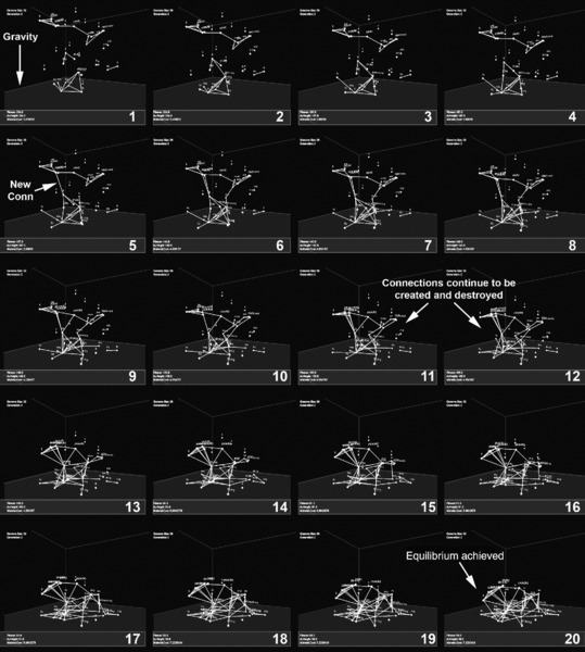
Figure 14.19 Solutions evolved within a simple physics simulation. Nodes are positioned within Cartesian space and contain growth instructions. During growth, nodes are subjected to gravity and “settle” to form a network solution.
To address these key issues, our recent work [56] extends our gene network using an alternative encoding method, replacing our cumbersome bit-string genomes with CPPNs [64], and this allows us to evolve scalable and regular designs for truss optimization problems. Additionally, further work [57] is now underway to explore the evolution of high-value structures for various engineering applications with additive manufacturing technologies (i.e., 3D printing).
ACKNOWLEDGMENTS
Daniel Richards was supported by funding from the Dalton Research Institute, Manchester Metropolitan University.
REFERENCES
- Aldana, M., Balleza, E., Kauffman, S., and Resendiz, O. 2007. Robustness and evolvability in genetic regulatory networks. Journal of Theoretical Biology, 245, 433–448.
- Bentley, P. J. and O’Reilly, U. M. 2001. Ten steps to make a perfect creative evolutionary design system. In Proceedings of GECCO ’01, Workshop on Non-Routine Design with Evolutionary Systems, San Francisco, July 7–11, 2001.
- Blondel, V. D., Guillaume, J. L., Lambiotte, R., and Lefebvre, E. 2008. Fast unfolding of communities in large networks, Journal of Statistical Mechanics, 10, doi:10.1088/1742-5468/2008/10/P10008.
- Bongard, J. and Pfeifer, R. 2003. Evolving complete agents using artificial ontogeny. In Hara, F. and Pfeifer, R (Eds), Morpho-Functional Machines: The New Species (Designing Embodied Intelligence), Berlin: Springer Verlag, pp. 237–258.
- Burry, M. 2011. Scripting Cultures: Architectural Design and Programming. Sussex: John Wiley & Sons.
- Caldas, L. G. 2001. An Evolution-Based Generative Design System: Using Adaptation to Shape Architectural Form. Ph.D. thesis, Massachussetts Institute of Technology.
- Caldas, L. 2008. Generation of energy-efficient architecture solutions applying GENE_ARCH: an evolution-based generative design system. Advanced Engineering Informatics, 22, 59–70.
- Clune, J. and Lipson, H. 2011. Evolving three-dimensional objects with a generative encoding inspired by developmental biology. In Proceedings of ECAL 2011, Paris, pp. 141–148.
- Collins, M. 2005. Finding needles in haystacks is harder with neutrality. In Proceedings of GECCO ’05, Washington, June 25–29, 1613–1618.
- Crombach, A. and Hogeweg, P. 2008. Evolution of evolvability in gene regulatory networks. PLoS Comput Biol, 4(7): e1000112. doi:10.1371/journal.pcbi.1000112
- Davis, D., Burry, M., and Burry, J. 2011. Untangling parametric schemata: enhancing collaboration through modular programming, In Proceedings of the 14th International Conference on Computer Aided Architectural Design Futures, Liege (Belgium), 4–8 July 2011, 55–68.
- Doncieux, S., Mouret, J. B., Bredeche, N., and Padois, V. 2011. Evolutionary Robotics: Exploring New Horizions. Studies in Computational Intelligence. Vol 341, Springer, pp. 3–25.
- Draghi, J. A., Parsons, T. L., Wagner, G. P., and Plotkin, J. B. 2010. Mutational robustness can facilitate adaptation. Nature Letters, 263, 353–355.
- Eggenberger, P. 1997. Evolving morphologies of simulated 3D organisms based on differential gene expression, In Husbands, P. and Harvey, I. (Eds), Proceedings of the Fourth European Conference on Artificial Life, Brighton, UK, July 28–31, 1997, MIT Press, pp. 205--213.
- Espinoso-Soto, C., Martin, O. C., and Wagner, A. 2011. Phenotype plasticity can facilitate adaptive evolution in gene regulatory circuits. BMC Evolutionary Biology, 11(5): doi:10.1186/1471-2148-11-5.
- Evins, R. 2013. A review of computational optimisation methods applied to sustainable building design. Renewable and Sustainable Energy Reviews, 22, 230–245.
- Flatt, T. 2005. The evolutionary genetics of canalization. The Quarterly Review of Biology, 80(3), 287–316.
- Forbes, P. 2006. The Gecko’s Foot: How Scientists are Taking a Leaf from Nature’s Book. London: Harper Perennial.
- Frazer, J. 1995. An Evolutionary Architecture. London, UK: Architectural Association.
- Galvan-Lopez, E., McDermott, J., O’Neil, M., and Brabazon, A. 2010. Towards an understanding of locality in genetic programming. In Proceedings of GECCO ’10, July 7–11, 2010, Portland, USA. ACM Press, 901–908.
- Galvan-Lopez, E., Poli, R., Kattan, A., O’Neil, M., and Brabazon, A. 2011. Neutrality in evolutionary algorithms what do we know? Evolving Systems 2(3), 145–163.
- Gibson, G. and Wagner, G. 2000. Canalization in evolutionary genetics: a stabilizing theory? BioEssays 22(4), 372–380.
- Glynn, R. and Sheil, B. (Eds). 2011. Fabricate: Making Digital Architecture. Ontario: Riverside Architectural Press.
- Harvey, I. and Thompson, A. 1997. Through the labyrinth evolution finds a way: a silicon ridge, In Higuchi, T. Iwata, M., and Liu, W. (Eds), Proceedings of 1st International Conference on Evolvable Systems: From Biology to Hardware, Berlin, Germany: Springer-Verlag, Vol. 1259, 406–422.
- Hayden, E. J., Ferrada, E., and Wagner, A. 2011. Cryptic genetic variation promotes rapid evolutionary adaptation in an RNA enzyme. Nature, 474(6), 92–95.
- Hensel, M., Menges, A., and Weinstock, M. 2010. Emergent Technologies and Design: Towards a Biological Paradigm for Architecture, Oxon: Routledge.
- Hornby, G. 2004. Functional scalability through generative representations: the evolution of table designs. Environment and Planning B, 3, 569–587.
- Hu, T., Payne, J. L., Banzhaf, W., and Moore, J. H. 2011. Robustness, evolvability and accessibility in linear genetic programming, In Silva, S., Foster, J., Nicolau, M., Machado, P., and Giacobini, M. (Eds), Proceedings of EuroGP 2011, Evostar, Springer’s Lecture Notes in Computer Science, vol. 6621, 13–24.
- Kauffman, S. A. 1993. The Origins of Order: Self?Organization and Selection in Evolution. Oxford: Oxford University Press.
- Kicinger, R., Arcissewski, T., and Jong, K. 2005. Evolutionary computation and structural design: a survey of the state of the art. Computers and Structures, 83, 1943–1978.
- Kimura, M. 1968. Evolutionary rate at the molecular level. Nature, 217, 624–626.
- Kitano, H. 2004. Biological robustness. Nature Reviews Genetics, 5(11), 826–837.
- Kumar, S. and Bentley, P. J. (Eds). 2003. On Growth, Form and Computers. London: Elsevier.
- Lenski, R. E., Barrick, J. E., and Ofria, C. 2006. Balancing robustness and evolvability, PLoS Biology, 4(12): e428. doi:10.1371/journal.pbio.0040428
- Le Rouzic, A. and Carlborg, O. 2007. Evolutionary potential of hidden genetic variation. TRENDS in Ecology and Evolution, 23(1), 33–37.
- Lipson, H. 2005. Evolutionary design and open ended design automation. Biomimetics, 129–155.
- Menges, A. 2012. Higher integration in morphogenetic design. Architectural Design, 82(2).
- Miller, J. F. 2003. Evolving developmental programs for adaptation, morphogenesis and self-repair, In Proceedings of ECAL ’03, Dortmund, 2003, 256–265.
- Miller, J. 2004. Evolving a self-repairing, self-regulating, french flag organism. In Proceedings of GECCO ’04, Washington, June 26–30, 129–139.
- Miller, J. F. 2011. Cartesian genetic programming, In Miller, J. F. (Ed), Cartesian Genetic Programming, Berlin: Springer Verlag, 17–34.
- Moore, S. A. 2007. Alternative Routes to the Sustainable City. Plymouth: Lexington Books.
- Muller, G. B. 2007. Evo-devo: extending the evolutionary synthesis. Nature Reviews Genetics, 8(12), 943–949.
- Newman, M. E. J. 2008. The mathematics of networks. In Blume and S. N. Durlauf (Eds.), The New Palgrave Encycolpedia of Economics, Basingstoke: Palgrave Macmillan.
- Nolfi, S. and Parisi, D. 1991. Growing neural networks (Tech. Rep. PCIA-91-15). Rome: Institute of Psychology, C.N.R.
- O’Neil, M., McDermott, J., Swafford, J. M., Byrne, J., Hemberg, E., Brabason, A., Shotton, E., McNally, C. and Hemberg, M. 2010. Evolutionary design using grammatical evolution and shape grammars: designing a shelter. International Journal of Design Engineering, 3(1), 4–24.
- O’Reilly, U. M. and Hemberg, M. 2007. Integrating generative growth and evolutionary computation for form exploration. Genetic Programming and Evolvable Machines, 8(2), 163–186.
- Oxman, N. 2010. Structuring materiality: design fabrication of heterogeneous materials. Architectural Design, 80(4), 78–85.
- Oxman, R. 2009. Performative design: a performance-based model of digital architectural design. Environment and Planning B: Planning and Design, 36, 1026–1037.
- Pask, G. 1969. The architectural relevance of cybernetics. Architectural Design, 7(6), 494–496.
- Pigliucci, M. 2008. Is evolvability evolvable? Nature Reviews Genetics, 9(1), 75–82.
- Raidl, G. R. and Gottlieb, J. 2005. Empirical analysis of locality heritability and heuristic bias in evolutionary algorithms: A case study for the multidimensional knapsack problem. Evolutionary Computation, 13(4), 441–414.
- Reisinger, J., Stanley, K. O., and Miikkulainen, R. 2005. Towards an empirical measure of evolvability, In Proceedings of GECCO ’05, June 25–29, 2005, Washington, DC, 257–264.
- Richards, D. 2011. Towards morphogenetic assemblies. In Herr, C.M., Gu, N., Roudavski, S., Schabel, M. A. (Eds), Circuit Bending, Breaking and Mending: Proceedings of the 16th International Conference on Computer-Aided Architectural Design Research in Asia (CAADRIA), 515–524.
- Richards, D. 2013. Automatic Synthesis of Architectural Structures using an Evo-Devo Approach to Design. Ph.D. thesis, Manchester Metropolitan University, UK.
- Richards, D., Dunn, N., and Amos, M. 2012. An evo-devo approach to architectural design. In Proceedings of GECCO 12, July 7–11, 2012, Philadelphia, USA. ACM Press, 569–576.
- Richards, D. and Amos, M. (2014a). Evolving morphologies with CPPN-NEAT and a dynamic substrate. In Hiroki Sayama, John Rieffel, Sebastian Risi, Ren Doursat and Hod Lipson (Eds), Proceedings of ALIFE 14, the Fourteenth International Conference on the Synthesis and Simulation of Living Systems, July 30–August 2, 2014, New York, USA., 255–262, MIT Press.
- Richards, D. and Amos, M. (2014b). Designing with gradients: bio-inspired computation for digital fabrication. Accepted for presentation at ACADIA 2014: Design Agency, October 23–25, 2014, University of Southern California, Los Angeles, USA.
- Rothlauf, F. and Goldberg, D. E. 2000. Pruefer numbers and genetic algorithms: a lesson on how the low locality of an encoding can harm the performance of GA’s. In Proceedings of the 6th International Conference on Parallel Problem Solving from Nature (PPSN), London: Springer Verlag, 395–404.
- Rothlauf, F. 2011. Design of Modern Heuristics Principles and Application. Heidelberg: Springer.
- Roudavski, S. 2009. Towards morphogenesis in architecture. International Journal of Architectural Computing, 7(3), 345–374.
- Rutherford, S. L. 2000. From genotype to phenotype: buffering mechanisms and the storage of genetic information. BioEssays, 22(12), 1095–1105.
- Siegal, M. L. and Bergman, A. 2002. Waddington’s canalization revisited: Developmental stability and evolution. Proceedings of the National Academy of Sciences of the United States of America, 99(16), 10528–10532.
- Stanley, K. O. and Miikkulainen, R. 2003. A taxonomy of artificial embryogeny, Artificial Life, 9(2), 93–130.
- Stanley, K. O. 2007. Compositional pattern producing networks: a novel abstraction of development. Genetic Programming and Evolvable Machines, 8(2), 131–162.
- Tanzer, K. and Longoria, R. (Eds). 2007. The Green Braid: Towards an Architecture of Ecology, Economy and Equity. Oxon: Routledge.
- Turrin, M., von Buelow, P., and Stouffs, R. 2011. Design explorations of performance driven geometry in architectural design using parametric modelling and genetic algorithms. Advanced Engineering Informatics, 25(4), 656–675.
- Ulieru, M. and Doursat, R. 2011. Emergent engineering: a radical paradigm shift. International Journal of Autonomous and Adaptive Communications Systems, 4(1), 39–60.
- van Dijk, A. D. J., van Mourik, S., and van Ham, R. C. H. J. 2012. Mutational robustness of gene regulatory networks. PLoS ONE, 7(1): e30591. doi:10.1371/journal.pone.0030591.
- Vassilev, V. K. and Miller, J. F. 2000. The advantages of landscape neutrality in digital circuit evolution, In Proceedings of ICES ’00, April 17–19, 2000, Edinburgh, 252–263.
- Waddington, C. H. 1942. Canalization of development and the inheritance of acquired characters. Nature, 150, 563.
- Waddington, C. H. 1957. The Strategy of the Genes: A Discussion of Some Aspects of Theoretical Biology. London: Allen and Unwin; New York: MacMillan.
- Wagner, A. 2005. Robustness, evolvability, and neutrality. FEBS Letters 579(8), 1772--1778.
- Wagner, A. 2011. The Origins of Evolutionary Innovation: A Theory of Transformative Change in Living Systems, Oxford: Oxford University Press.
- Wagner, A. 2012. The role of robustness in phenotypic adaptation and innovation, Proceedings of the Royal Society B: Biological Sciences, 279, 1249–125.
- Watson, J. D., Baker, T. A., Bell, S. P., Gann, A., Levine, M., and Losick, R. 2007. Molecular Biology of the Gene. New York: Benjamin Cummings.
- Weinstock, M. 2006. Self-organisation and the structural dynamics of plants, Architectural Design, 76(2), 26–33.
- Yu. T. and Miller. J F. 2002. Finding needles in haystacks is not hard with neutrality. In Foster, J. A., Lutton, E., Miller, J. F., Ryan, C., and Tezzamanzi, A. G. B. (Eds), Proceedings of EuroGP 2002. LNCS, Vol 2278, 13–25.