6

Integration

In this chapter we discuss numerical integration, a basic tool of scientific computation. We derive the Simpson and trapezoid rules but just sketch the basis of Gaussian quadrature, which, though our standard workhorse, is long in derivation. We do discuss Gaussian quadrature in its various forms and indicate how to transform the Gauss points to a wide range of intervals. We end the chapter with a discussion of Monte Carlo integration, which is fundamentally different from other integration techniques.

6.1  Integrating a Spectrum (Problem)

Problem: An experiment has measured dN(t)/dt, the number of particles per unit time entering a counter. Your problem is to integrate this spectrum to obtain the number of particles N (1) that entered the counterin thefirst second foran arbitrary decay rate

6.2  Quadrature as Box Counting (Math)

The integration of a function may require some cleverness to do analytically but is relatively straightforward on a computer. A traditional way to perform numerical integrationbyhandis totakea pieceof graph paper and count the numberofboxes or quadrilaterals lying below a curveof the integrand. For this reason numerical integration isalso callednumerical quadrature even when it becomes more sophisticated than simple box counting.

The Riemann definition of an integral is the limit of the sum over boxes as the width h of the box approaches zero (Figure 6.1):

Figure 6.1 The integral ¡a f(x) dx is the area under the graph of f(x) from a to b. Here we break up the area into four regions of equal widths h.

The numerical integral of a function f(x) is approximated as the equivalent of a finite sum over boxes of height f (x) and width wi:

which is similar to the Riemann definition (6.2) except that there is no limit to an infinitesimal box size. Equation (6.3) is the standard form for all integration algorithms; the function f(x) is evaluated at N points in the interval [a, b], and the function values fi = f (xi) are summed with each term in the sum weighted by wi. While in general the sum in (6.3) gives the exact integral only when N —> oo, it may be exact for finite N if the integrand is a polynomial. The different integration algorithms amount to different ways of choosing the points and weights. Generally the precision increases as N gets larger, with round-off error eventually limiting the increase. Because the “best” approximation depends on the specific behavior of f (x), there is no universally best approximation. In fact, some of the automated integration schemes found in subroutine libraries switch from one method to another and change the methods for different intervals until they find ones that work well for each interval.

In general you should not attempt a numerical integration of an integrand that contains a singularity without first removing the singularity by hand.¹ You may be able to do this very simply by breaking the interval down into several subintervals so the singularity is at an endpoint where an integration point is not placed or by a change of variable:

Likewise,ifyour integrand has a very slow variation in some region, you can speed up the integration by changing to a variable that compresses that region and places few points there. Conversely, if your integrand has a very rapid variation in some region, you may want to change to variables that expand that region to ensure that no oscillations are missed.

6.2.1  Algorithm: Trapezoid Rule

The trapezoid and Simpson integration rules use values of f(x) at evenly spaced values of x. They use N points xi(i = 1,N) evenly spaced at a distance h apart throughout the integration region [a, b] and include the endpoints. This means that there are (N - 1) intervals of length h:

where we start our counting at i = 1. The trapezoid rule takes each integration interval i and constructs a trapezoid of width h in it (Figure 6.2). This approximates f(x) by a straight line in each interval i and uses the average height (fi + fi₊₁)/2 as the value for f. The area of each such trapezoid is

In terms of our standard integration formula (6.3), the “rule” in (6.8) is for N = 2 points with weights wi ≡ ¹₂ (Table 6.1).

In order to apply the trapezoid rule to the entire region [a, b], we add the contributions from each subinterval:

Figure 6.2 Right: Straight-line sections used for the trapezoid rule. Left: Two parabolas used in Simpson’s rule.

You will notice that because the internal points are counted twice (as the end of one interval and as the beginning of the next), they have weights of h/2 +h/2 = h, whereas the endpoints are counted just once and on that account have weights of only h/2. In terms of our standard integration rule (6.32), we have

In Listing 6.1 we provide a simple implementation of the trapezoid rule.

6.2.2  Algorithm: Simpson’s Rule

For each interval, Simpson’s rule approximates the integrand f(x) by a parabola (Figure 6.2 right):

TABLE 6.1
Elementary Weights for Uniform-Step Integration Rules

Name	Degree	Elementary Weights
Trapezoid	1	(1, 1)h2
Simpson’s	2	(1, 4, 1)h3
	3	(1, 3, 3, 1) 38 h
Milne	4	(14, 64,24, 64,14) 4h5

Listing 6.1 Trap.java integrates the function t² via the trapezoid rule. Note how the step size h depends on the interval and how the weights at the ends and middle differ.

with all intervals equally spaced. The area under the parabola for each interval is

In order to relate the parameters α, β, and γ to the function, we consider an interval from -1 to +1, in which case

But we notice that

In this way we can express the integral as the weighted sum over the values of the function at three points:

Because three values of the function are needed, we generalize this result to our problem by evaluating the integral over two adjacent intervals, in which case we evaluate the function at the two endpoints and in the middle (Table 6.1):

Simpson’s rule requires the elementary integration to be over pairs of intervals, which in turn requires that the total number of intervals be even or that the number of points N be odd. In order to apply Simpson’s rule to the entire interval, we add up the contributions from each pair of subintervals, counting all but the first and last endpoints twice:

In terms of our standard integration rule (6.3), we have

The sum of these weights provides a useful check on your integration:

Remember, the number of points N must be odd for Simpson’s rule.

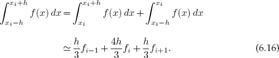
6.2.3  Integration Error (Analytic Assessment)

In general, you should choose an integration rule that gives an accurate answer using the least number of integration points. We obtain a crude estimate of the approximation or algorithmic error E and the relative error e by expanding f (x) in a Taylor series around the midpoint of the integration interval. We then multiply that error by the number of intervals N to estimate the error for the entire region [a, b]. For the trapezoid and Simpson rules this yields

We see that the third-derivative term in Simpson’s rule cancels (much like the central-difference method does in differentiation). Equations (6.20) are illuminating in showing how increasing the sophistication of an integration rule leads to an error that decreases with a higher inverse power of N, yet is also proportional to higher derivatives of f. Consequently, for small intervals and functions f(x) with well-behaved derivatives, Simpson’s rule should converge more rapidly than the trapezoid rule.

To model the error in integration, we assume that after N steps the relative round off error is random and of the form

where em is the machine precision, e 10-7 for single precision and e 10-15 for double precision (the standard for science). Because most scientific computations are done with doubles, we will assume double precision. We want to determine an N that minimizes the total error, that is, the sum of the approximation and round-off errors:

This occurs, approximately, when the two errors are of equal magnitude, which we approximate even further by assuming that the two errors are equal:

To continue the search for optimum N for a general function f, we set the scale of function size and the lengths by assuming

The estimate (6.23), when applied to the trapezoid rule, yields

The estimate (6.23), when applied to Simpson’s rule, yields

These results are illuminating in that they show how

6.2.4  Algorithm: Gaussian Quadrature

It is often useful to rewrite the basic integration formula (6.3) such that we separate a weighting function W(x) from the integrand:

In the Gaussian quadrature approach to integration, the N points and weights are chosen to make the approximation error vanish if g(x) were a (2N -1)-degree polynomial. To obtain this incredible optimization, the points xi end up having a specific distribution over [a, b]. In general, if g(x) is smooth or can be made smooth by factoring out some W(x) (Table 6.2), Gaussian algorithms will produce higher accuracy than the trapezoid and Simpson rules for the same number of points. Sometimes the integrand may not be smooth because it has different behaviors in different regions. In these cases it makes sense to integrate each region separately and then add the answers together. In fact, some “smart” integration subroutines decide for themselves how many intervals to use and what rule to use in each.

All the rules indicated in Table 6.2 are Gaussian with the general form (6.31). We can see that in one case the weighting function is an exponential, in another a

TABLE 6.2
Types of Gaussian Integration Rules

TABLE 6.3
Points and Weights for four-point Gaussian Quadrature

±yi	wi
0.33998 10435 84856	0.65214 51548 62546
0.86113 63115 94053	0.34785 48451 37454

Gaussian, and in several an integrable singularity. In contrast to the equally spaced rules, there is never an integration point at the extremes of the intervals, yet the values of the points and weights change as the number of points N changes. Although we will leave the derivation of the Gaussian points and weights to the references on numerical methods, we note here that for ordinary Gaussian (Gauss-Legendre) integration, the points yi turn out to be the N zeros of the Leg-endre polynomials, with the weights related to the derivatives, PN(yi) = 0, and wi = 2/([(1 — yi ²)[PN(yi)]2]. Subroutines to generate these points and weights are standard in mathematical function libraries, are found in tables such as those in [A&S 72], or can be computed. The gauss subroutines we provide on the CD (available online: http://press.princeton.edu/landau_survey/) also scale the points to span specified regions. As a check that your points are correct, you may want to compare them to the four-point set in Table 6.3.

6.2.4.1 MAPPING INTEGRATION POINTS

Our standard convention (6.3) for the general interval [a, b] is

With Gaussian points and weights, the y interval — 1 < yi < 1 must be mapped onto the x interval a <x <b. Here are some mappings we have found useful in our work. In all cases (yi,wi) are the elementary Gaussian points and weights for the interval [—1,1], and we want to scale to x with various ranges.

6.2.5  Integration Implementation and Error Assessment

In Listing 6.2 we give a sample program that performs an integration with Gaussian points. The method gauss generates the points and weights and may be useful in other applications as well.

Listing 6.2 IntegGauss.java integrates the function f(x) via Gaussian quadrature. The points and weights are generated in the method gauss,which remains fixed for all applications. Note that the parameter eps, which controls the level of precision desired, should be set by the user,as should the value for job,which controls the mapping of the Gaussian points onto arbitrary intervals (they are generated for -1 ≤ x ≤ 1).

6.3  Experimentation

Try two integrals for which the answers are less obvious:

Explain why the computer may have trouble with these integrals.

6.4  Higher-Order Rules (Algorithm)

As in numerical differentiation, we can use the known functional dependence of the error on interval size h to reduce the integration error. For simple rules like the trapezoid and Simpson rules, we have the analytic estimates (6.23), while for others you may have to experiment to determine the h dependence. To illustrate, if A(h) and A(h/2) are the values of the integral determined for intervals h and h/2, respectively, and we know that the integrals have expansions with a leading error term proportional to h²,

Consequently, we make the h² term vanish by computing the combination

Clearly this particular trick (Romberg’s extrapolation) works only if the h² term dominates the error and then only if the derivatives of the function are well behaved. An analogous extrapolation can also be made for other algorithms.

In Table 6.1 we gave the weights for several equal-interval rules. Whereas the Simpson rule used two intervals, the three-eighths rule uses three, and the Milne² rule four. (These are single-interval rules and must be strung together to obtain a rule extended over the entire integration range. This means that the points that end one interval and begin the next are weighted twice.) You can easily determine the number of elementary intervals integrated over, and check whether you and we have written the weights right, by summing the weights for any rule. The sum is the integral of f(x) = 1 and must equal h times the number of intervals (which in turn equals b-a):

6.5  Problem: Monte Carlo Integration by Stone Throwing

Imagine yourself as a farmer walking to your furthermost field to add algae-eating fish to a pond having an algae explosion. You get there only to read the instructions and discover that you need to know the area of the pond in order to determine the correct number of the fish to add. Your problem is to measure the area of this irregularly shaped pond with just the materials at hand [G,T&C 06].

It is hard to believe that Monte Carlo techniques canbe used to evaluate integrals. After all, we do not want to gamble on the values! While it is true that other methods are preferable for single and double integrals, Monte Carlo techniques are best when the dimensionality of integrations gets large! For our pond problem, we will use a sampling technique (Figure 6.4):

6.5.1  Stone Throwing Implementation

Use sampling (Figure 6.4) to perform a 2-D integration and thereby determine π:

6.5.2  Integration by Mean Value (Math)

The standard Monte Carlo technique for integration is based on the mean value theorem (presumably familiar from elementary calculus):

The theorem states the obvious if you think of integrals as areas: The value of the integral of some function f (x) between a and b equals the length of the interval (b — a) times the mean value of the function over that interval (f} (Figure 6.5). The integration algorithm uses Monte Carlo techniques to evaluate the mean in (6.45). With a sequence a < x¿ < b of N uniform random numbers, we want to determine the sample mean by sampling the function f (x) at these points:

Figure 6.5 The area under the curve f (x) is the same as that under the dashed line y = (f).

This gives us the very simple integration rule:

Equation (6.47) looks much like our standard algorithm for integration (6.3) with the “points” xi chosen randomly and with uniform weights wi = (b — a)/N. Because no attempt has been made to obtain the best answer for a given value of N, this is by no means an optimized way to evaluate integrals; but you will admit it is simple. If we let the number of samples of f (x) approach infinity N —> oo or if we keep the number of samples finite and take the average of infinitely many runs, the laws of statistics assure us that (6.47) will approach the correct answer, at least if there were no round-off errors.

For readers who are familiar with statistics, we remind you that the uncertainty in the value obtained for the integral I after N samples of f(x) is measured by the standard deviation σ¡. If σj is the standard deviation of the integrand f in the sampling, then for normal distributions we have

So for large N, the error in the value obtained for the integral decreases as 1/ N.

6.6  High-Dimensional Integration (Problem)

Let’s say that we want to calculate some properties of a small atom such as magnesium with 12 electrons. To do that we need to integrate atomic wave functions over the three coordinates of each of 12 electrons. This amounts to a 3×12 = 36-D integral. If we use 64 points for each integration, this requires about 6436 1065 evaluations of the integrand. If the computer were fast and could evaluate the integrand a billion times per second, this would take about 1056 s, which is significantly longer than the age of the universe (^1017 s).

Your problem is to find a way to perform multidimensional integrations so that you are still alive to savor the answers. Specifically, evaluate the 10-D integral

Check your numerical answer against the analytic one, ¹⁵₆⁵.

6.6.1  Multidimensional Monte Carlo

It is easy to generalize mean value integration to many dimensions by picking random points in a multidimensional space. For example,

6.6.2  Error in Multidimensional Integration (Assessment)

When we perform a multidimensional integration, the error in the Monte Carlo technique, being statistical, decreases as 1/yN. This is valid even if the N points are distributed over D dimensions. In contrast, when we use these same N points to perform a D-dimensional integration as D 1-D integrals using a rule such as Simpson’s, we use N/D points for each integration. For fixed N, this means that the number of points used for each integration decreases as the number of dimensions D increases, and so the error in each integration increases with D. Furthermore, the total error will be approximately N times the error in each integral. If we put these trends together and look at a particular integration rule, we will find that at a value of D 3-4 the error in Monte Carlo integration is similar to that of conventional schemes. For larger values of D, the Monte Carlo method is always more accurate!

6.6.3  Implementation: 10-D Monte Carlo Integration

Use a built-in random-number generator to perform the 10-D Monte Carlo integration in (6.49). Our program Int10d.java is available on the instructor’s CD (available online: http://press.princeton.edu/landau_survey/).

6.7  Integrating Rapidly Varying Functions (Problem)

It is common in many physical applications to integrate a function with an approximately Gaussian dependence on x. The rapid falloff of the integrand means that our Monte Carlo integration technique would require an incredibly large number of points to obtain even modest accuracy. Your problem is to make Monte Carlo integration more efficient for rapidly varying integrands.

6.7.1  Variance Reduction (Method)

If the function being integrated never differs much from its average value, then the standard Monte Carlo mean value method (6.47) should work well with a large, but manageable, number of points. Yet for a function with a large variance (i.e., one that is not “flat”), many of the random evaluationsof the function may occur where the function makes a slight contribution to the integral; this is, basically, a waste of time. The method can be improved by mapping the function f into a function g that has a smaller variance over the interval. We indicate two methods here and refer you to [Pres 00] and [Koon 86] for more details.

The first method is a variance reduction or subtraction technique in which we devise a flatter function on which to apply the Monte Carlo technique. Suppose we construct a function g(x) with the following properties on [a, b]:

We now evaluate the integral of f(x)-g(x) and add the result to J to obtain the required integral

If we are clever enough to find a simple g(x) that makes the variance of f(x)-g(x) less than that of f(x) and that we can integrate analytically, weobtain more accurate answers in less time.

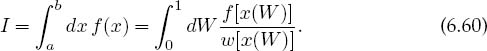
6.7.2  Importance Sampling (Method)

A second method for improving Monte Carlo integration is called importance sampling because it lets us sample the integrand in the most important regions. It derives from expressing the integral in the form

If wenow use w(x) as theweighting functionor probability distribution for our random numbers, the integral can be approximated as

The improvement from (6.54) is that a judicious choice of weighting function w(x) ∝ f (x) makes f(x)/w(x) more constant and thus easier to integrate.

6.7.3  Von Neumann Rejection (Method)

A simple, ingenious method for generating random points with a probability distribution w(x) was deduced by von Neumann. This method is essentially the same as the rejection or sampling method used to guess the area of a pond, only now the pond has been replaced by the weighting function w(x), and the arbitrary box around the lake by the arbitrary constant WQ. Imagine a graph of w(x) versus x (Figure 6.6). Walk off your box by placing the line W = WQ on the graph, with the only condition being WQ ≥ w(x). We next “throw stones” at this graph and count only those that fall into the w(x) pond. That is, we generate uniform distributions in x and y ≡ W with the maximum y value equal to the width of the box WQ:

We then reject all xi that do not fall into the pond:

The xi values so accepted will have the weighting w(x) (Figure 6.6). The largest acceptance occurs where w(x) is large, in this case for midrange x. In Chapter 15, “Thermodynamic Simulations & Feynman Quantum Path Integration,” we apply a variation of the rejection technique known as the Metropolis algorithm. This algorithm has now become the cornerstone of computation thermodynamics.

6.7.4  Simple Gaussian Distribution

The central limit theorem can be used to deduce a Gaussian distribution via a simple summation. The theorem states, under rather general conditions, that if {ri} is a

Figure 6.6 The Von Neumann rejection technique for generating random points with weight w(x).

sequence of mutually independent random numbers, then the sum

is distributed normally. This means that the generated x values have the distribution

6.8  Nonuniform Assessment Θ

Use the von Neumann rejection technique to generate a normal distribution of standard deviation 1 and compare to the simple Gaussian method.

6.8.1  Implementation: Nonuniform Randomness

In order for w(x) to be the weighting function for random numbers over [a, b], we want it to have the properties

where dP is the probability of obtaining an x in the range x->x + dx. For the uniform distribution over [a, b], w(x) = 1/(b — a).

Inverse transform/change of variable method ©: Let us consider a change of variables that takes our original integral I (6.53) to the form

Our aim is to make this transformation such that there are equal contributions from all parts of the range in W; that is, we want to use a uniform sequence of random numbers for W. To determine the new variable, we start with u(r), the uniform distribution over [0, 1],

We want to find a mapping rfixor probability function w(x) for which probability is conserved:

This means that even though x and r are related by some (possibly) complicated mapping, x is also random with the probability of x lying in x —> x + dx equal to that of r lying in r —> r + dr.

To find the mapping between x and r (the tricky part), we change variables to W(x) defined by the integral

We recognize W(x) as the (incomplete) integral of the probability density u(r) up to some point x. It is another type of distribution function, the integrated probability of finding a random number less than the value x. The function W(x) is on that account called a cumulative distribution function and can also be thought of as the area to the left of r = x on the plot of u(r) versus r. It follows immediately from the definition (6.63) that W(x) has the properties

Consequently, Wi = {ri} is a uniform sequence of random numbers, and we just need to invert (6.63) to obtain x values distributed with probability w(x).

The crux of this technique is being able to invert (6.63) to obtain x = W-¹(r). Let us look at some analytic examples to get a feel for these steps (numerical inversion is possible and frequent in realistic cases).

Uniform weight function w: We start with the familiar uniform distribution

After following the rules, this leads to

where W(x) is always taken as uniform. In this way we generate uniform random 0 ≤ r ≤ 1 and uniform random a ≤ x ≤ b.

Exponential weight: We want random points with an exponential distribution:

In this way we generate uniform random r: [0,1] and obtain x = – λln(1 -r) distributed with an exponential probability distribution for x > 0. Notice that our prescription (6.53) and (6.54) tells us to use w(x) = e~x/λ/λ to remove the exponential-like behavior from an integrand and place it in the weights and scaled points (0 < xi < ∞). Because the resulting integrand will vary less, it may be approximated better as a polynomial:

Gaussian (normal) distribution: We want to generate points with a normal distribution:

This by itself is rather hard but is made easier by generating uniform distributions in angles and then using trigonometric relations to convert them to a Gaussian distribution. But before doing that, we keep things simple by realizing that we can obtain (6.71) with mean x and standard deviation σ by scaling and a translation of a simpler w(x):

We start by generalizing the statement of probability conservation for two different distributions (6.62) to two dimensions [Pres 94]:

We recognize the term in vertical bars as the Jacobian determinant:

To specialize to a Gaussian distribution, we consider 2πr as angles obtained from a uniform random distribution r, and x and y as Cartesian coordinates that will have a Gaussian distribution. The two are related by

The inversion of this mapping produces the Gaussian distribution

The solution to our problem is at hand. We use (6.74) with r₁ and r₂ uniform random distributions, and x and y are then Gaussian random distributions centered around x = 0.

1 In Chapter 20, “Integral Equations in Quantum Mechanics,” we show how to remove such a singularity even when the integrand is unknown.

2 There is, not coincidentally, a Milne Computer Center at Oregon State University, although there no longer is a central computer there.