12

Discrete & Continuous Nonlinear Dynamics

Nonlinear dynamics is one of the success stories of computational science. It has been explored by mathematicians, scientists, and engineers, with computers as an essential tool. The computations have led to the discovery of new phenomena such as solitons, chaos, and fractals, as you will discover on your own. In addition, because biological systems often have complex interactions and may not be in thermodynamic equilibrium states, models of them are often nonlinear, with properties similar to those of other complex systems.

In Unit I we develop the logistic map as a model for how bug populations achieve dynamic equilibrium. It is an example of a very simple but nonlinear equation producing surprising complex behavior. In Unit II we explore chaos for a continuous system, the driven realistic pendulum. Our emphasis there is on using phase space as an example of the usefulness of an abstract space to display the simplicity underlying complex behavior. In Unit III we extend the discrete logistic map to nonlinear differential models of coupled predator–prey populations and their corresponding phase space plots.

12.1  Unit I. Bug Population Dynamics (Discrete)

Problem: The populations of insects and the patterns of weather do not appear to follow any simple laws.¹ At times they appear stable, at other times they vary periodically, and at other times they appear chaotic, only to settle down to something simple again. Your problem is to deduce if a simple, discrete law can produce such complicated behavior.

12.2  The Logistic Map (Model)

Imagine a bunch of insects reproducing generation after generation. We start with N₀ bugs, then in the next generation we have to live with N₁ of them, and after i generations there are Ni bugs to bug us. We want to define a model of how Nn varies with the discrete generation number n. For guidance, we look to the radioactive decay simulation in Chapter 5, “Monte Carlo Simulations”, where the discrete decay law, ∆N/∆t = —λN, led to exponential-like decay. Likewise, if we reverse the sign of λ, we should get exponential-like growth, which is a good place to start our modelling. We assume that the bug-breeding rate is proportional to the number of bugs:

Because we know as an empirical fact that exponential growth usually tapers off, we improve the model by incorporating the observation that bugs do not live on love alone; they must also eat. But bugs, not being farmers, must compete for the available food supply, and this might limit their number to a maximum N* (called the carrying capacity). Consequently, we modify the exponential growth model (12.1) by introducing a growth rate λ’ that decreases as the population Ni approaches N* :

We expect that when Ni is small compared to N*, the population will grow exponentially, but that as Ni approaches N*, the growth rate will decrease, eventually becoming negative if Ni exceeds N*, the carrying capacity.

Equation (12.2) is one form of the logistic map. It is usually written as a relation between the number of bugs in future and present generations:

The map looks simple when expressed in terms of natural variables:

where µ is a dimensionless growth parameter and xi is a dimensionless population variable. Observe that the growth rate µ equals 1 when the breeding rate λ’ equals 0, and is otherwise expected to be larger than 1. If the number of bugs born per generation λ’ ∆ t is large, then µ λ’ ∆tN* and xi Ni/N.,.. That is, xi is essentially a fraction of the carrying capacity N*. Consequently, we consider x values in the range 0 < xi < 1, where x = 0 corresponds to no bugs and x = 1 to the maximum population. Note that there is clearly a linear, quadratic dependence of the RHS of (12.5) on xi. In general, a map uses a function f(x) to map one number in a sequence to another,

For the logistic map, f (x) = µx(1 — x), with the quadratic dependence of f on x making this a nonlinear map, while the dependence on only the one variable xi makes it a one-dimensional map.

12.3  Properties of Nonlinear Maps (Theory)

Rather than do some fancy mathematical analysis to determine the properties of the logistic map [Rash 90], we prefer to have you study it directly on the computer by plotting xi versus generation number i. Some typical behaviors are shown in Figure 12.1. In Figure 12.1A we see equilibration into a single population; in Figure 12.1B we see oscillation between two population levels; in Figure 12.1C we see oscillation among four levels; and in Figure 12.1D we see a chaotic system. The initial population xQ is known as the seed, and as long as it is not equal to zero, its exact value usually has little effect on the population dynamics (similar to what we found when generating pseudorandom numbers). In contrast, the dynamics are unusually sensitive to the value of the growth parameter µ. For those values of µ at which the dynamics are complex, there may be extreme sensitivity to the initial condition xQ as well as to the exact value of µ.

12.3.1  Fixed Points

An important property of the map (12.5) is the possibility of the sequence xi reaching a fixed point at which xi remains or fluctuates about. We denote such fixed points as x-,_. At a one-cycle fixed point, there is no change in the population from generation i to generation i + 1; that is,

Using the logistic map (12.5) to relate xi₊₁ to xi yields the algebraic equation

The nonzero fixed point x-,_ = (µ — 1) /µ corresponds to a stable population with a balance between birth and death that is reached regardless of the initial population (Figure 12.1A). In contrast, the x* = 0 point is unstable and the population remains static only as long as no bugs exist; if even a few bugs are introduced, exponential growth occurs. Further analysis (§12.8) tells us that the stability of a population is determined by the magnitude of the derivative of the mapping function f(xi) at the fixed point [Rash 90]:

Figure 12.1 The insect population xn versus the generation number n for various growth rates. (A) µ = 2.8,a single attractor. If the fixed point is xn = 0, the system becomes extinct. (B) µ = 3.3,a double attractor. (C) µ = 3.5,a quadruple attractor. (D) µ = 3.8,a chaotic regime. If µ < 1,the population goes extinct.

the fixed point [Rash 90]:

For the one cycle of the logistic map (12.5), we have

12.3.2  Period Doubling, Attractors

Equation (12.11) tells us that while the equation for fixed points (12.9) may be satisfied for all values of µ, the populations will not be stable if µ > 3. For µ > 3, the system’s long-term population bifurcates into two populations (a two-cycle), an effect known as period doubling (Figure 12.1B). Because the system now acts as if it were attracted to two populations, these populations are called attractors or cycle points. We can easily predict the x values for these two-cycle attractors by demanding that generation i +2 have the same population as generation i:

We see that as long as µ > 3, the square root produces a real number and thus that physical solutions exist (complex or negative x* values are nonphysical). We leave it to your computer explorations to discover how the system continues to double periods as µ continues to increase. In all cases the pattern is the same: One of the populations bifurcates into two.

12.4  Mapping Implementation

Program the logistic map to produce a sequence of population values x¿ as a function of the generation number i. These are called map orbits. The assessment consists of confirmation of Feigenbaum’s observations [Feig 79] of the different behavior patterns shown in Figure 12.1. These occur for growth parameter µ = (0.4, 2.4,3.2, 3.6,3.8304) and seed population x0 = 0.75. Identify the following on your graphs:

12.5  Bifurcation Diagram (Assessment)

Computing and watching the population change with generation number gives a good idea of the basic dynamics, at least until it gets too complicated to discern patterns. In particular, as the number of bifurcations keeps increasing and the system becomes chaotic, it is hard for us to see a simple underlying structure within the complicated behavior. One way to visualize what is going on is to concentrate on the attractors, that is, those populations that appear to attract the solutions and to which the solutions continuously return. A plot of these attractors (long-term iterates) of the logistic map as a function of the growth parameter µ is an elegant way to summarize the results of extensive computer simulations.

A bifurcation diagram for the logistic map is given in Figure 12.2, while one for a Gaussian map is given in Figure 12.3. For each value of µ, hundreds of iterations are made to make sure that all transients essentially die out, and then the values (µ, x*) are written to a file for hundreds of iterations after that. If the system falls into an n cycle for this µ value, then there should predominantly be n different values written to the file. Next, the value of the initial populations xo is changed slightly, and the entire procedure is repeated to ensure that no fixed points are missed. When finished, your program will have stepped through all the values of growth parameter µ, and for each value of µ it will have stepped through all the values of the initial population xQ. Our sample program Bugsjava is shown in Listing 12.1.

Listing 12.1 Bugs.java, the basis of a program for producing the bifurcation diagram of the logistic map. A finished program requires finer grids, a scan over initial values, and removal of duplicates.

Figure 12.2 The bifurcation plot, attractor populations versus growth rate, for the logistic map. The inset shows some details of a three-cycle window.

12.5.1  Bifurcation Diagram Implementation

The last part of this problem is to reproduce Figure 12.2 at various levels of detail. (You can listen to a sonification of this diagram on the CD or use one of the applet there to create your own sonification.) While the best way to make a visualization of this sort would be with visualization software that permits you to vary the intensity of each individual point on the screen, we simply plot individual points and have the density in each region determined by the number of points plotted there. When thinking about plotting many individual points to draw a figure, it is important to keep in mind that your screen resolution is ^100 dots per inch and your laser printer resolution may be 300 dots per inch. This means that if you plot a point at each pixel, you will be plotting ^3000 χ 3000^10 million elements. Beware: This can require some time and may choke a printer. In any case, printing at a finer resolution is a waste of time.

12.5.2  Visualization Algorithm: Binning

12.5.3  Feigenbaum Constants (Exploration)

Feigenbaum discovered that the sequence of µ^ values (12.13) at which bifurcations occur follows a regular pattern [Feig 79]. Specifically, it converges geometrically when expressed in terms of the distance between bifurcations δ:

Use your sequence of µk values to determine the constants in (12.14) and compare them to those found by Feigenbaum:

Amazingly, the value of the Feigenbaum constant δ is universal for all second-order maps.

12.6  Random Numbers via Logistic Map (Exploration)

There are claims that the logistic map in the chaotic region (µ > 4),

can be used to generate random numbers [P&R 95]. Although successive xi’s are correlated, if the population for approximately every sixth generation is examined, the correlation is effectively gone and random numbers result. To make the sequence more uniform, a trigonometric transformation is used:

Use the random-number tests discussed in Chapter 5, “Monte Carlo Simulation,” to test this claim.

TABLE 12.1
Several Nonlinear Maps to Explore

Name	f(x)	Name	f(x)
Logistic	µx(1-x)	Tent	µ(1 - 2 |x - 1/2|)
Ecology	xeµ(1-x)	Quartic	µ[1-(2x - 1)4]
Gaussian	ebx2 +µ

12.7  Other Maps (Exploration)

Bifurcations and chaos are characteristic properties of nonlinear systems. Yet systems can be nonlinear in a number of ways. Table 12.1 lists four maps that generate xi sequences containing bifurcations. The tent map derives its nonlinear dependence from the absolute value operator, while the logistic map is a subclass of the ecology map. Explore the properties of these other maps and note the similarities and differences.

12.8  Signals of Chaos: Lyapunov Coefficients

The Lyapunov coefficient λi provides an analytic measure of whether a system is chaotic [Wolf 85, Ram 00, Will 97]. Physically, the coefficient is a measure of the growth rate of the solution near an attractor. For 1-D maps there is only one such coefficient, whereas in general there is a coefficient for each direction in space. The essential assumption is that neighboring paths xn near an attractor have an n (or time) dependence L oc exp(λt). Consequently, orbits that have λ > 0 diverge and are chaotic; orbits that have λ = 0 remain marginally stable, while orbits with λ < 0 are periodic and stable. Mathematically, the Lyapunov coefficient or exponent is defined as

where L(t) is the distance between neighboring phase space trajectories at time t.

We calculate the Lyapunov exponent for a general 1-D map,

and then apply the result to the logistic map. To determine stability, we examine perturbations about a reference trajectory x₀ by adding a small perturbation and iterating once [Mann 90, Ram 00]:

We substitute this into (12.19) and expand f in a Taylor series around x₀:

(This is the proof of our earlier statement about the stability of maps.) To deduce the general result we examine one more iteration:

This last relation tells us how trajectories differ on the average after n steps:

We now solve for the Lyapunov number L and take its logarithm to obtain the Lyapunov exponent:

For the logistic map we obtain

where the sum is over iterations.

The code LyapLog.java in Listing 12.2 computes the Lyapunov exponents for the bifurcation plot of the logistic map. In Figure 12.4 left we show its output and note the sign changes in λ where the system becomes chaotic, and abrupt changes in slope at bifurcations. (A similar curve is obtained for the fractal dimension of the logistic map, as indeed the two are proportional.)

12.8.1  Shannon Entropy

Shannon entropy, like the Lyapunov exponent, is another analytic measure of chaos. It is a measure of uncertainty that has proven useful in communication theory

Listing 12.2 LyapLog.java computes Lyapunov exponents for the bifurcation plot of the logistic map as a function of growth rate. Note the fineness of the μ grid.

[Shannon 48, Ott 02, G,T&C 06] and led to the concept of information entropy. Imagine that an experiment has N possible outcomes. If the probability of each is p1,p2,…,pN, with normalization such that ¿^i₌₁ pi = 1, the Shannon entropy is defined as

If pi = 0, there is no uncertainty and Shannon = 0, as you might expect. If all N outcomes have equal probability, pi = 1/N, we obtain SShannon = ln N, which diverges slowly as N —» oo.

The code Entropy.java in Listing 12.3 computes the Shannon entropy for the the logistic map as a function of the growth parameter µ. The results (Figure 12.4 left) are seen to be quite similar to the Lyapunov exponent, again with discontinuities occurring at the bifurcations.

12.9  Unit I Quiz

Listing 12.3 Entropy.java computes the Shannon entropy for the logistic map as a function of growth parameter µ.

12.10  Unit II. Pendulums Become Chaotic (Continuous)

In Unit I on bugs we discovered that a simple nonlinear difference equation yields solutions that may be simple, complicated, or chaotic. Unit III will extend that model to the differential form, which also exhibits complex behaviors. Now we search for similar nonlinear, complex behaviors in the differential equation describing a realistic pendulum. Because chaotic behavior may resemble noise, it is important to be confident that the unusual behaviors arise from physics and not numerics. Before we explore the solutions, we provide some theoretical background on the use of phase space plots for revealing the beauty and simplicity underlying complicated behaviors. We also provide two chaotic pendulum applets (Figure 12.5) for assistance in understanding the new concepts. Our study is based on the description in [Rash 90], on the analytic discussion of the parametric oscillator in [L&L,M 76], and on a similar study of the vibrating pivot pendulum in [G,T&C 06].

Consider the pendulum on the left in Figure 12.5. We see a pendulum of length l driven by an external sinusoidal torque f through air with a coefficient of drag α. Because there is no restriction that the angular displacement θ be small, we call this a realistic pendulum. Your problem is to describe the motion of this pendulum, first when the driving torque is turned off but the initial velocity is large enough to send the pendulum over the top, and then when the driving torque is turned on.

12.11  Chaotic Pendulum ODE

What we call a chaotic pendulum is just a pendulum with friction and a driving torque (Figure 12.5 left) but with no small-deflection-angle approximation. Newton’s laws of rotational motion tell us that the sum of the gravitational torque -mgl sin θ, the frictional torque -βθ, and the external torque τQ cos ωt equals the moment of inertia of the pendulum times its angular acceleration [Rash 90]:

Equation (12.29) is a second-order time-dependent nonlinear differential equation. Its nonlinearity arises from the sinθ, as opposed to the θ, dependence of the gravitational torque. The parameter ω₀ is the natural frequency of the system arising from the restoring torque, α is a measure of the strength of friction, and f is a measure of the strength of the driving torque. In our standard ODE form, dy/dt = y (Chapter 9, “Differential Equation Applications”), we have two simultaneous first-order equations:

Figure 12.5 Left: A pendulum of length l driven through air by an external sinusoidal torque. The strength of the torque is given by f and that of air resistance by α. Right: A double pendulum.

12.11.1  Free Pendulum Oscillations

If we ignore friction and external torques, (12.29) takes the simple form

If the displacements are small, we can approximate sinθ by θ and obtain the linear equation of simple harmonic motion with frequency ω₀:

In Chapter 9, “Differential Equation Applications,” we studied how nonlinearities produce anharmonic oscillations, and indeed (12.33) is another good candidate for such studies. As before, we expect solutions of (12.33) for the free realistic pendulum to be periodic, but with a frequency ω ~ ω ₀ only for small oscillations. Furthermore, because the restoring torque, mgl sin θ ~ mgl(θ – θ3/3), is less than the mglθ assumed in a harmonic oscillator, realistic pendulums swing slower (have longer periods) as their angular displacements are made larger.

12.11.2  Solution as Elliptic Integrals

The analytic solution to the realistic pendulum is a textbook problem [L&L,M 76, M&T 03, Schk 94], except that it is hardly a solution and hardly analytic. The “solution” is based on energy being a constant (integral) of the motion. For simplicity, we start the pendulum off at rest from its maximum displacement θm. Because the initial energy is all potential, we know that the total energy of the system equals its initial potential energy (Figure 12.5),

Yet since E = KE+PE is a constant, we can write for any value of θ

where we have assumed that it takes T/4 for the pendulum to travel from θ = 0 to θm. The integral in (12.36) is an elliptic integral of the first kind. If you think of an elliptic integral as a generalization of a trigonometric function, then this is a closed-form solution; otherwise, it’s an integral needing computation. The series expansion of the period (12.37) is obtained by expanding the denominator and

integrating it term by term. It tells us, for example, that an amplitude of 80° leads to a 10% slowdown of the pendulum relative to the small θ result. In contrast, we will determine the period empirically without the need for any expansions.

12.11.3  Implementation and Test: Free Pendulum

As a preliminary to the solution of the full equation (12.29), modify your rk4 program to solve (12.33) for the free oscillations of a realistic pendulum.

12.12  Visualization: Phase Space Orbits

The conventional solution to an equation of motion is the position x(t) and the velocity v(t) as functions of time. Often behaviors that appear complicated as functions of time appear simpler when viewed in an abstract space called phase space, where the ordinate is the velocity v(t) and the abscissa is the position x(t) (Figure 12.7). As we see from the phase space figures, the solutions form geometric objects that are easy to recognize. (We provide two applets on the CD (available online: http://press.princeton.edu/landau_survey/), Pend1 and Pend2, to help the reader make the connections between phase space shapes and the corresponding physical motion.)

Figure 12.6 The data screen (left) and output screen (right) of the applet HearData on the CD. Columns of (ti,x(ti)) data are pasted into the data window, processed into the graph in the output window, and then converted to sound that is played by Java.

The position and velocity of a free harmonic oscillator are given by the trigonometric functions

When substituted into the total energy, we obtain two important results:

The first equation, being that of an ellipse, proves that the harmonic oscillator follows closed elliptical orbits in phase space, with the size of the ellipse increasing with the system’s energy. The second equation proves that the total energy is a constant of the motion. Different initial conditions having the same energy start at different places on the same ellipse and transverse the same orbits.

In Figures 12.7–12.10 we show various phase space structures. Study these figures and their captions and note the following:

12.12.1  Chaos in Phase Space

It is easy to solve the nonlinear ODE (12.31) on the computer using our usual techniques. However, it is not so easy to understand the solutions because they are so rich in complexity. The solutions are easier to understand in phase space, particularly if you learn to recognize some characteristic structures there. Actually, there are a number of “tools” that can be used to decide if a system is chaotic in contrast to just complex. Geometric structures in phase space is one of them, and determination of the Lyupanov coefficient (discussed in §12.8) is another. Both signal the simplicity lying within the complexity.

Figure 12.8 Left: Phase space trajectories for a plane (i.e. 2-D) pendulum including “over the top” or rotating solutions. The trajectories are symmetric with respect to vertical and horizontal reflections through the origin. At the bottom of the figure is shown the corresponding θ dependence of the potential. Right: Position versus time for two initial conditions of a chaotic pendulum that end up with the same limit cycle,and the corresponding phase space orbits. (Courtesy of W. Hager.)

What may be surprising is that even though the ellipselike figures in phase space were observed originally for free systems with no friction and no driving torque, similar structures continue to exist for driven systems with friction. The actual trajectories may not remain on a single structure for all times, but they are attracted to them and return to them often. In contrast to periodic motion, which corresponds to closed figures in phase space, random motion appears as a diffuse cloud filling an entire energetically accessible region. Complex or chaotic motion falls someplace in between (Figure 12.9 middle). If viewed for long times and for many initial conditions, chaotic trajectories (flows) through phase space, while resembling the familiar geometric figures, they may contain dark or diffuse bands in places rather than single lines. The continuity of trajectories within bands means that a continuum of solutions is possible and that the system flows continuously among the different trajectories forming the band. The transitions among solutions cause the coordinate space solutions to appear chaotic and are what makes them hypersensitive to the initial conditions (the slightest change in which causes the system to flow to nearby trajectories).

Pick out the following phase space structures in your simulations.

Limit cycles: When a chaotic pendulum is driven by a not-too-large driving torque, it is possible to pick the magnitude for this torque such that after the initial transients die off, the average energy put into the system during one period exactly balances the average energy dissipated by friction during that period (Figure 12.8 right):

Figure 12.9 Position and phase space plots for a chaotic pendulum with ω₀ = 1,α = 0.2, f = 0.52, and ω = 0.666. The rightmost initial condition displays more of the broadband Fourier spectrum characteristic of chaos. (Examples of chaotic behavior can be seen in Figure 12.10.)

This leads to limit cycles that appear as closed ellipselike figures, yet the solution may be unstable and make sporadic jumps between limit cycles.

Predictable attractors: Well-defined, fairly simple periodic behaviors that are not particularly sensitive to the initial conditions. These are orbits, such as fixed points and limit cycles, into which the system settles or returns to often. If your location in phase space is near a predictable attractor, ensuing times will bring you to it.

Strange attractors: Well-defined, yet complicated, semiperiodic behaviors that appear to be uncorrelated with the motion at an earlier time. They are distinguished from predicable attractors by being fractal (Chapter 13, “Fractals & Statistical Growth”) chaotic, and highly sensitive to the initial conditions [J&S 98]. Even after millions of oscillations, the motion remains attracted to them.

Figure 12.10 Some examples of complicated behaviors of a realistic pendulum. In the top three rows sequentially we see θ(t) behaviors,a phase space diagram containing regular patterns with dark bands, and a broad Fourier spectrum. These features are characteristic of chaos. In the bottom two rows we see how the behavior changes abruptly after a slight change in the magnitude of the force and that for f = 0.54 there occur the characteristic broad bands of chaos.

Chaotic paths: Regions of phase space that appear as filled-in bands rather than lines. Continuity within the bands implies complicated behaviors, yet still with simple underlying structure.

Mode locking:When the magnitude f of the driving torque is larger than that for a limit cycle (12.41), the driving torque can overpower the natural oscillations, resulting in a steady-state motion at the frequency of the driver. This is called mode locking. While mode locking can occur for linear or nonlinear systems, for nonlinear systems the driving torque may lock onto the system by exciting its overtones, leading to a rational relation between the driving frequency and the natural frequency:

Butterfly effects: One of the classic quips about the hypersensitivity of chaotic systems to the initial conditions is that the weather pattern in North America is hard to predict well because it is sensitive to the flapping of butterfly wings in South America. Although this appears to be counterintuitive because we know that systems with essentially identical initial conditions should behave the same, eventually the systems diverge. The applet pend2 (Figure 12.11 bottom) lets you compare two simulations of nearly identical initial conditions.As seen on the right in Figure 12.11, the initial conditions for both pendulums differ by only 1 part in 917, and so the initial paths in phase space are the same. Nonetheless, at just the time shown here, the pendulums balance in the vertical position, and then one falls before the other, leading to differing oscillations and differing phase space plots from this time onward.

12.12.2  Assessment in Phase Space

The challenge in understanding simulations of the chaotic pendulum (12.31) is that the 4-D parameter space (ω₀, α,f,ω) is so immense that only sections of it can be studied systematically. We expect that sweeping through driving frequency ω should show resonances and beating; sweeping through the frictional force α should show underdamping, critical damping, and overdamping; and sweeping through the driving torque f should show mode locking (for the right values of ω). All these behaviors can be found in the solution of your differential equation, yet they are mixed together in complex ways.

In this assessment you should try to reproduce the behaviors shown in the phase space diagrams in Figure 12.9 and in the applets in Figure 12.11. Beware: Because the system is chaotic, you should expect that your results will be sensitive to the exact values of the initial conditions and to the details of your integration routine. We suggest that you experiment; start with the parameter values we used to produce our plots and then observe the effects of making very small changes in parameters until you obtain different modes of behavior. Consequently, an inability to reproduce our results fortheparametervalues does not necessarilyimply thatsomething is “wrong.”

Figure 12.11 Top row: Output from the applet Pend1 producing an animation of a chaotic pendulum, along with the corresponding position versus time and phase space plots. Right: The resulting Fourier spectrum produced by Pend1,Bottom row: Output from the applet Pend2 producing an animation of two chaotic pendula,along with the corresponding phase space plots, and the final output with limit cycles (dark bands).

12.13  Exploration: Bifurcations of Chaotic Pendulums

We have seen that a chaotic system contains a number of dominant frequencies and that the system tends to “jump” from one to another. This means that the dominant frequencies occur sequentially, in contrast to linear systems where they occur simultaneously. We now want to explore this jumping as a computer experiment. If we sample the instantaneous angular velocity θ = dθ/dt of our chaotic simulation at various instances in time, we should obtain a series of values for the frequency, with the major Fourier components occurring more often than others.³ These are the frequencies to which the system is attracted. That being the case, if we make a scatterplot of the sampled θs for many times at one particular value of the driving force and then change the magnitude of the driving force slightly and sample the frequencies again, the resulting plot may show distinctive patterns of frequencies. That a bifurcation diagram similar to the one for bug populations results is one of the mysteries of life.

Figure 12.12 A bifurcation diagram for the damped pendulum with a vibrating pivot (see also the similar diagram for a double pendulum, Figure 12.14). The ordinate is |dθ/dt|, the absolute value of the instantaneous angular velocity at the beginning of the period of the driver, and the abscissa is the magnitude of the driving force f. Note that the heavy line results from the overlapping of points,not from connecting the points (see enlargement in the inset).

In the scatterplot in Figure 12.12, we sample θ for the motion of a chaotic pendulum with a vibrating pivot point (in contrast to our usual vibrating external torque). This pendulum is similar to our chaotic one (12.29), but with the driving force depending on sin θ:

Essentially, the acceleration of the pivot is equivalent to a sinusoidal variation of g or ωQ. Analytic [L&L,M 76, § 25-30] and numeric [DeJ 92, G,T&C 06] studies of this system exist. To obtain the bifurcation diagram in Figure 12.12:

Figure 12.13 Photographs of a double pendulum built by a student in the OSU Physics Department. The longer pendulum consists of two separated shafts so that the shorter one can rotate through it. Both pendula can go over the top. We see the pendulum released from rest and then moving quickly. The flash photography stops the motion in various stages. (Photograph,R. Landau.)

12.14  Alternative Problem: The Double Pendulum

For those of you who have already studied a chaotic pendulum, an alternative is to study a double pendulum without any small-angle approximation (Figure 12.5 right and Fig. 12.13, and animation DoublePend.mpg on the CD (available online: http://press.princeton.edu/landau_survey/)).A double pendulum has a second pendulum connected to the first, and because each pendulum acts as a driving force for the other, we need not include an external driving torque to produce a chaotic system (there are enough degrees of freedom without it).

The equations of motions for the double pendulum are derived most directly from the Lagrangian formulation of mechanics. The Lagrangian is fairly simple but has the θ₁ and θ₂ motions innately coupled:

Figure 12.14 Left: Phase space trajectories for a double pendulum with m₁ = 10m₂,showing two dominant attractors. Right: A bifurcation diagram for the double pendulum displaying the instantaneous velocity of the lower pendulum as a function of the mass of the upper pendulum. (Both plots are courtesy of J. Danielson.)

The resulting dynamic equations couple the θ₁ and θ₂ motions:

Usually textbooks approximate these equations for small oscillations, which diminish the effects of the coupling. “Slow” and “fast” modes then result for in-phase and antiphase oscillations, respectively, that look much like regular harmonic motions. What’s more interesting is the motion that results without any small-angle restrictions, particularly when the pendulums have enough initial energy to go over the top (Figure 12.13). On the left in Figure 12.14 we see several phase space plots for the lower pendulum with m1 = 10m2. When given enough initial kinetic energy to go over the top, the trajectories are seen to flow between two major attractors as energy is transferred back and forth to the upper pendulum.

On the right in Figure 12.14 is a bifurcation diagram for the double pendulum. This was created by sampling and plotting the instantaneous angular velocity θ ˙2 of the lower pendulum at 70 times as the pendulum passed through its equilibrium position. The mass of the upper pendulum (a convenient parameter) was then changed, and the process repeated. The resulting structure is fractal and indicates bifurcations in the number of dominant frequencies in the motion. A plot of the Fourier or wavelet spectrum as a function of mass is expected to show similar characteristic frequencies.

12.15  Assessment: Fourier/Wavelet Analysis of Chaos

We have seen that a realistic pendulum experiences a restoring torque, τg ∝ sin θ ~ θ – θ3/3! + θ5/5! + •••, that contains nonlinear terms that lead to nonharmonic behavior. In addition, when a realistic pendulum is driven by an external sinusoidal torque, the pendulum may mode-lock with the driver and so oscillate at a frequency that is rationally related to the driver’s. Consequently, the behavior of the realistic pendulum is expected to be a combination of various periodic behaviors, with discrete jumps between modes.

In this assessment you should determine the Fourier components present in the pendulum’s complicated and chaotic behaviors. You should show that a three-cycle structure, for example, contains three major Fourier components, while a five-cycle structure has five. You should also notice that when the pendulum goes over the top, its spectrum contains a steady-state (DC) component.

Wavelet Exploration: We saw in Chapter 11, “Wavelet Analysis & Data Compression”, that a wavelet expansion is more appropriate than a Fourier expansion for a signal containing components that occur for finite periods of time. Because chaotic oscillations are just such signals, repeat the Fourier analysis of this section using wavelets instead of sines and cosines. Can you discern the temporal sequence of the various components?

12.16  Exploration: Another Type of Phase Space Plot

Imagine that you have measured the displacement of some system as a function of time. Your measurements appear to indicate characteristic nonlinear behaviors, and you would like to check this by making a phase space plot but without going to the trouble of measuring the conjugate momenta to plot versus displacement. Amazingly enough, one may also plot x(t + τ) versus x(t) as a function of time to obtain a phase space plot [Abar 93]. Here τ is a lag time and should be chosen as some fraction of a characteristic time for the system under study. While this may not seem like a valid way to make a phase space plot, recall the forward difference approximation for the derivative,

We see that plotting x(t + τ) versus x(t) is equivalent to plotting v(t) versus x(t).

Exercise: Create a phase space plot from the output of your chaotic pendulum by plotting θ(t + τ) versus θ(t) for a large range of t values. Explore how the graphs change for different values of the lag time τ. Compare your results to the conventional phase space plots you obtained previously.

12.17  Further Explorations

12.18  Unit III. Coupled Predator–Prey Models

In Unit I we saw complicated behavior arising from a model of bug population dynamics in which we imposed a maximum population. We described that system with a discrete logistic map. In Unit II we saw complex behaviors arising from differential equations and learned how to use phase space plots to understand them. In this unit we study the differential equation model describing Predator–Prey population dynamics proposed by the American physical chemist Lotka [Lot 25] and the Italian mathematician Volterra [Volt 26]. Differential equations are easy to solve numerically and should be a good approximation if populations are large. However, there are equivalent discrete map versions of the model as well. Though simple, versions of these equations are used to model biological systems and neural networks.

Problem: Is it possible to use a small number of predators to control a population of pests so that the number of pests remains approximately constant? Include in your considerations the interaction between the populations as well as the competition for food and predation time.

12.19  Lotka–Volterra Model

We extend the logistic map to the Lotka–Volterra Model (LVM) to describe two populations coexisting in the same geographical region. Let

In the absence of interactions between the species, we assume that the prey population p breeds at a per-capita rate of a, which would lead to exponential growth:

Yet exponential growth does not occur because the predators P eat more preyas the prey numbers increase. The interaction rate between predator and prey requires both to be present, with the simplest assumption being that it is proportional to their joint probability:

Interaction rate = bpP.

This leads to a prey growth rate including both predation and breeding:

If left to themselves, predators P will also breed and increase their population. Yet predators need animals to eat, and if there are no other populations to prey upon, they will eat each other (or their young) at a per-capita mortality rate m:

However, once there are prey to interact with (read “eat”) at the rate bpP, the predator population will grow at the rate

Figure 12.15 The populations of prey p and predator P from the Lotka-Volterra model. Left: The time dependences of the prey p(t) (solid) and the predators P(t) (dashed). Right: Prey population p versus predator population P. The different orbits in this “phase space plot” correspond to different initial conditions.

where e is a constant that measures the efficiency with which predators convert prey interactions into food.

Equations (12.55) and (12.57) are two simultaneous ODEs and are our first model. We solve them with the rk4 algorithm of Chapter 9, “Differential Equation Applications”, after placing them in the standard dynamic form,

A sample code to do this is PredatorPrey.java and is given on the CD (available online: http://press.princeton.edu/landau_survey/). Results from our solution are shown in Figure 12.15. On the left we see that the two populations oscillate out of phase with each other in time; when there are many prey, the predator population eats them and grows; yet then the predators face a decreased food supply and so their population decreases; that in turn permits the prey population to grow, and so forth. On the right in Figure 12.15 we plot a phase space plot (phase space plots are discussed in Unit II) of P(t) versus p(t). A closed orbit here indicates a limit cycle that repeats indefinitely. Although increasing the initial number of predators does decrease the maximum number of pests, it is not a satisfactory solution to our problem, as the large variation in the number of pests cannot be called control.

12.19.1  LVM with Prey Limit

The initial assumption in the LVM that prey grow without limit in the absence of predators is clearly unrealistic. As with the logistic map, we include a limit on prey numbers that accounts for depletion of the food supply as the prey population grows. Accordingly, we modify the constant growth rate a → a(1- p/K) so that growth vanishes when the population reaches a limit K, the carrying capacity,

The behavior of this model with prey limitations is shown in Figure 12.16. We see that both populations exhibit damped oscillations as they approach their equilibrium values. In addition, and as hoped for, the equilibrium populations are independent of the initial conditions. Note how the phase space plot spirals inward to a single close limit cycle, on which it remains, with little variationinprey number. This is control, and we may use it to predict the expected pest population.

12.19.2  LVM with Predation Efficiency

An additional unrealistic assumption in the original LVM is that the predators immediately eat all the prey with which they interact.As anyone who has watched a cat hunt a mouse knows, predators spend time finding prey and also chasing, killing, eating, and digesting it (all together called handling). This extra time decreases the rate bpP at which prey are eliminated. Wedefine the functional response pa as the probability of one predator finding one prey. If a single predator spends time t_search searching for prey, then

If we call th the time a predator spends handling a single prey, then the effective time a predator spends handling a prey is pa th. Such being the case, the total time T that a predator spends finding and handling a single prey is

where pa/T is the effective rate of eating prey. We see that as the number of prey p → ∞, the efficiency in eating them → 1. We include this efficiency in (12.59) by modifying the rate b at which a predator eliminates prey to b/(1 +bpth):

Figure 12.16 The Lotka–Volterra model of prey population p and predator population P with a prey population limit. Left: The time dependences of the prey p(t) (solid) and the predators P(t) (dashed). Right: Prey population p versus predator population P.

To be more realistic about the predator growth, we also place a limit on the predator carrying capacity but make it proportional to the number of prey:

Solutions for the extended model (12.61) and (12.62) are shown in Figure 12.17. Observe the existence of three dynamic regimes as a function of b:

The transition from equilibrium to a limit cycle is called a phase transition.

We finally have a satisfactory solution to our problem. Although the prey population is not eliminated, it can be kept from getting too large and from fluctuating widely. Nonetheless, changes in the parameters can lead to large fluctuations or to nearly vanishing predators.

12.19.3  LVM Implementation and Assessment

1.  Write a program to solve (12.61) and (12.62) using the rk4 algorithm and the following parameter values.

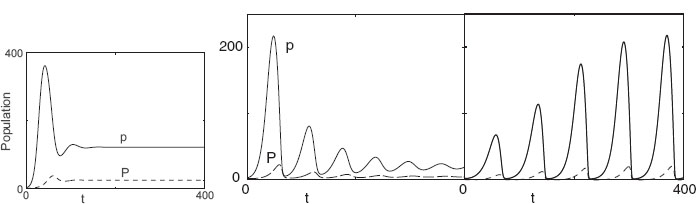
Figure 12.17 Lotka–Volterra model with predation efficiency and prey limitations. From left to right: overdamping,b = 0.01; damped oscillations,b = 0.1,and limit cycle,b = 0.3.

Model	a	b	e	m	K	k
LVM-I	0.2	0.1	1	0.1	0	—
LVM-II	0.2	0.1	1	0.1	20.0	—
LVM-III	0.2	0.1	—	0.1	500.0	0.2

12.19.4  Two Predators, One Prey (Exploration)

1 Except maybe in Oregon, where storm clouds come to spend their weekends.

2 You may recall from Chapter 5, “Monte Carlo Simulations,” that a random sequence of events does not even have step-by-step correlations.

3 We refer to this angular velocity as θ since we have already used ω for the frequency of the driver and ωQ for the natural frequency.