16

Simulating Matter with Molecular Dynamics

Problem: Determine whether a collection of argon molecules placed in a box will form an ordered structure at low temperature.

You may have seen in your introductory classes that the ideal gas law can be derived from first principles if gas molecules are treated as billiard balls bouncing off the walls but not interacting with each other. We want to extend this model so that we can solve for the motion of every molecule in a box interacting with every other molecule via a potential. We picked argon because it is an inert element with a closed shell of electrons and so can be modeled as almost-hard spheres.

16.1 Molecular Dynamics (Theory)

Molecular dynamics (MD) is a powerful simulation technique for studying the physical and chemical properties of solids, liquids, amorphous materials, and biological molecules. Even though we know that quantum mechanics is the proper theory for molecular interactions, MD uses Newton’s laws as the basis of the technique and focuses on bulk properties, which do not depend much on small-r behaviors. In 1985 Car and Parrinello showed how MD can be extended to include quantum mechanics by applying density functional theory to calculate the force [C&P 85]. This technique, known as quantum MD, is an active area of research but is beyond the realm of the present chapter.¹ For those with more interest in the subject, there are full texts [A&T 87, Rap 95, Hock 88] on MD and good discussions [G,T&C 06, Thij 99, Fos 96], as well as primers [Erco] and codes, [NAMD, Mold, ALCMD] available on-line.

MD’s solution of Newton’s laws is conceptually simple, yet when applied to a very large number of particles becomes the “high school physics problem from hell.” Some approximations must be made in order not to have to solve the 10²³–10²⁵ equations of motion describing a realistic sample but instead to limit the problem to ∼10⁶ particles for protein simulations and ∼10⁸ particles for materials simulations. If we have some success, then it is a good bet that the model will improve if we incorporate more particles or more quantum mechanics, something that becomes easier as computing power continues to increase.

In a number of ways, MD simulations are similar to the thermal Monte Carlo simulations we studied in Chapter 15, “Thermodynamic Simulations & Feynman Quantum Path Integration,” Both typically involve a large number N of interacting particles that start out in some set configuration and then equilibrate into some dynamic state on the computer. However, in MD we have what statistical mechanics calls a microcanonical ensemble in which the energy E and volume V of the N particles are fixed. We then use Newton’s laws to generate the dynamics of the system. In contrast, Monte Carlo simulations do not start with first principles but instead incorporate an element of chance and have the system in contact with a heat bath at a fixed temperature rather than keeping the energy E fixed. This is called a canonical ensemble.

Because a system of molecules is dynamic, the velocities and positions of the molecules change continuously, and so we will need to follow the motion of each molecule in time to determine its effect on the other molecules, which are also moving. After the simulation has run long enough to stabilize, we will compute time averages of the dynamic quantities in order to deduce the thermodynamic properties. We apply Newton’s laws with the assumption that the net force on each molecule is the sum of the two-body forces with all other (N -1) molecules:

In writing these equations we have ignored the fact that the force between argon atoms really arises from the particle–particle interactions of the 18 electrons and the nucleus that constitute each atom (Figure 16.1). Although it may be possible to ignore this internal structure when deducing the long-range properties of inert elements, it matters for systems such as polyatomic molecules that display rotational, vibrational, and electronic degrees of freedom as the temperature is raised.²

We assume that the force on molecule i derives from a potential and that the potential is the sum of central molecule–molecule potentials:

Here r_ij = |ri -rj| = r_ji is the distance between the centers of molecules i and j, and the limits on the sums are such that no interaction is counted twice. Because we have assumed a conservative potential, the total energy of the system, that is, the potential plus kinetic energies summed over all particles, should be conserved over time. Nonetheless, in a practical computation we “cut the potential off” [assume u(r_ij) = 0] when the molecules are far apart. Because the derivative of the potential produces an infinite force at this cutoff point, energy will no longer be precisely conserved. Yet because the cutoff radius is large, the cutoff occurs only when the forces are minuscule, and so the violation of energy conservation should be small relative to approximation and round-off errors.

Figure 16.1 The molecule–molecule effective interaction arises from the many-body interaction of the electrons and nucleus in one electronic cloud with the electrons and nucleus in another electron cloud. (The size of the nucleus at the center is highly exaggerated relative to the size of the molecule, and the electrons are really just points.)

In a first-principles calculation, the potential between any two argon atoms arises from the sum over approximately 1000 electron–electron and electron–nucleus Coulomb interactions. A more practical calculation would derive an effective potential based on a form of many-body theory, such as Hartree–Fock or density functional theory.Our approach is simpler yet. Weuse the Lennard–Jones potential,

TABLE 16.1
Parameter Values and Scales for the Lennard-Jones Potential

Figure 16.2 The Lennard-Jones potential. Note the sign change at r= 1 and the minimum at r 1.1225 (natural units). Note too that because the r axis does not extend to r= 0,the very high central repulsion is not shown.

Here the parameter ε governs the strength of the interaction, and σ determines the length scale. Both are deduced by fits to data, which is why this is called a “phenomenological” potential.

Some typical values for the parameters, and corresponding scales for the variables, are given in Table 16.1. In order to make the program simpler and to avoid under- and overflows, it is helpful to measure all variables in the natural units formed by these constants. The interparticle potential and force then take the forms

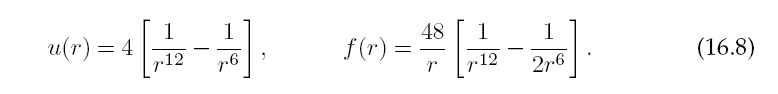
The Lennard-Jones potential is seen in Figure 16.2 to be the sum of a long-range attractive interaction ∝ 1/r⁶ and a short-range repulsive one ∝ 1/r12. The change from repulsion to attraction occurs at r = σ. The minimum of the potential occurs atr = 2¹/⁶σ = 1.1225σ, which would be the atom-atom spacing in a solid bound by this potential. The repulsive 1/r¹² term in the Lennard-Jones potential (16.6) arises when the electron clouds from two atoms overlap, in which case the Coulomb interaction and the Pauli exclusion principle keep the electrons apart. The 1/r¹² term dominates at short distances and makes atoms behave like hard spheres. The precise value of 12 is not of theoretical significance (although it’s being large is) and was probably chosen because it is 2 × 6.

The 1/r⁶ term dominates at large distances and models the weak van der Waals induced dipole-dipole attraction between two molecules.³ The attraction arises from fluctuations in which at some instant in time a molecule on the right tends to be more positive on the left side, like a dipole ⇐. This in turn attracts the negative charge in a molecule on its left, thereby inducing a dipole ⇐ in it. As long as the molecules stay close to each other, the polarities continue to fluctuate in synchronization ⇐⇐ so that the attraction is maintained. The resultant dipole–dipole attraction behaves like 1/r⁶, and although much weaker than a Coulomb force, it is responsible for the binding of neutral, inert elements, such as argon for which the Coulomb force vanishes.

16.1.1 Connection to Thermodynamic Variables

We assume that the number of particles is large enough to use statistical mechanics to relate the results of our simulation to the thermodynamic quantities (the simulation is valid for any number of particles, but the use of statistics requires large numbers). The equipartition theorem tells us that for molecules in thermal equilibrium at temperature T, each molecular degree of freedom has an energy k_BT/2 on the average associated with it, where kB = 1.38×10-²³ J/K is Boltzmann’s constant. A simulation provides the kinetic energy of translation⁴:

The time average of KE (three degrees of freedom) is related to temperature by

The system’s pressure P is determined by a version of the Virial theorem,

where the Virial w is a weighted average of the forces. Note that because ideal gases have no interaction forces, their Virial vanishes and we have the ideal gas law. The pressure is thus

where ρ = N/V is the density of the particles.

Figure 16.3 Left: Two frames from the animation of a 1-D simulation that starts with uniformly spaced atoms. Note how an image atom has moved in from the bottom after an atom leaves from the top. Right: Two frames from the animation of a 2-D simulation showing the initial and an equilibrated state. Note how the atoms start off in a simple cubic arrangement but then equilibrate to a face-centered-cubic lattice. In all cases, it is the interatomic forces that constrain the atoms to a lattice.

16.1.2 Setting Initial Velocity Distribution

Even though we start the system off with a velocity distribution characteristic of some temperature, since the system is not in equilibrium initially (some of the assigned KE goes into PE), this is not the true temperature of the system [Thij 99]. Note that this initial randomization is the only place where chance enters into our MD simulation, and it is there to speed the simulation along. Once started, the time evolution is determined by Newton’s laws, in contrast to Monte Carlo simulations which are inherently stochastic. We produce a Gaussian (Maxwellian) velocity distribution with the methods discussed in Chapter 5, “Monte Carlo Simulations.” In our sample code we take the average of uniform random numbers 0 ≤ r i ≤ 1 to produce a Gaussian distribution with mean <r> = 0.5. We then subtract this mean value to obtain a distribution about 0.

16.1.3 Periodic Boundary Conditions and Potential Cutoff

It is easy to believe that a simulation of 10²³ molecules should predict bulk properties well, but with typical MD simulations employing only 10³-10⁶ particles, one must be clever to make less seem like more. Furthermore, since computers are finite, the molecules in the simulation are constrained to lie within a finite box, which inevitably introduces artificial surface effects from the walls. Surface effects are particularly significant when the number of particles is small because then a large fraction of the molecules reside near the walls. For example, if 1000 particles are arranged ina10x10x10x10 cube, there are 10³-8³ = 488 particles one unit from the surface, that is, 49% of the molecules, while for 10⁶ particles this fraction falls to 6%.

Figure 16.4 The infinite space generated by imposing periodic boundary conditions on the particles within the simulation volume (shaded box). The two-headed arrows indicate how a particle interacts with the nearest version of another particle, be that within the simulation volume or an image. The vertical arrows indicate how the image of particle 4 enters when particle 4 exits.

The imposition of periodic boundary conditions (PBCs) strives to minimize the shortcomings of both the small numbers of particles and of artificial boundaries. Even though we limit our simulation to an Lx ×Ly ×Lz box, we imagine this box being replicated to infinity in all directions (Figure 16.4). Accordingly, after each time-integration step we examine the position of each particle and check if it has left the simulation region. If it has, then we bring an image of the particle back through the opposite boundary (Figure 16.4):

Consequently, each box looks the same and has continuous properties at the edges. As shown by the one-headed arrows in Figure 16.4, if a particle exits the simulation volume, its image enters from the other side, and so balance is maintained.

In principle a molecule interacts with all others molecules and their images, so even though there is a finite number of atoms in the interaction volume, there is an effective infinite number of interactions [Erco]. Nonetheless, because the Lennard-Jones potential falls off so rapidly for large r, V(r = 3σ) V(1.13σ)/200, far-off molecules do not contribute significantly to the motion of a molecule, and we pick a value r_cut 2.5σ beyond which we ignore the effect of the potential:

Accordingly, if the simulation region is large enough for u(r > Li/2) 0, an atom interacts with only the nearest image of another atom.

The only problem with the cutoff potential (16.14) is that since the derivative du/dr is singular at r = r_cut, the potential is no longer conservative and thus energy conservation is no longer ensured. However, since the forces are already very small at r_cut, the violation will also be very small.

16.2 Verlet and Velocity-Verlet Algorithms

A realistic MD simulation may require integration of the 3-D equations of motion for 10¹⁰ time steps for each of 10³-10⁶ particles. Although we could use our standard rk4 ODE solver for this, time is saved by using a simple rule embedded in the program. The Verlet algorithm uses the central-difference approximation (Chapter 7, “Differentiation & Searching”) for the second derivative to advance the solutions by a single time step h for all N particles simultaneously:

where we have set m = 1. (Improved algorithms may vary the time step depending upon the speed of the particle.) Notice that even though the atom–atom force does not have an explicit time dependence, we include a t dependence in it as a way of indicating its dependence upon the atoms’ positions at a particular time. Because this is really an implicit time dependence, energy remains conserved.

Part of the efficiency of the Verlet algorithm (16.16) is that it solves for the position of each particle without requiring a separate solution for the particle’s velocity. However, once we have deduced the position for various times, we can use the central-difference approximation for the first derivative of ri to obtain the velocity:

Note, finally, that because the Verlet algorithm needs r from two previous steps, it is not self-starting and so we start it with the forward difference,

Velocity-Verlet Algorithm: Another version of the Verlet algorithm, which we recommend because of its increased stability, uses a forward-difference approximation for the derivative to advance both the position and velocity simultaneously:

Although this algorithm appears to be of lower order than (16.16), the use of updated positions when calculating velocities, and the subsequent use of these velocities, make both algorithms of similar precision.

Of interest is that (16.21) approximates the average force during a time step as [Fi(t + h) +Fi(t)]/2. Updating the velocity is a little tricky because we need the force at time t+h, which depends on the particle positions at t+h. Consequently, we must update all the particle positions and forces to t+h before we update any velocities, while saving the forces at the earlier time for use in (16.21). As soon as the positions are updated, we impose periodic boundary conditions to ensure that we have not lost any particles, and then we calculate the forces.

16.3 1-D Implementation and Exercise

On the CD (available online: http://press.princeton.edu/landau_survey/) you will find a folder MDanimations that contains a number of 2-D animations (movies) of solutions to the MD equations. Some frames from these animations are shown in Figure 16.3. We recommend that you look at them in order to better visualize what the particles do during an MD simulation. In particular, these simulations use a potential and temperature that should lead to a solid or liquid system, and so you should see the particles binding together.

Listing 16.1 MD.java performs a 1-D MD simulation with too small a number of large time steps for just a few particles. To be realistic the user should change the parameters and the number of random numbers added to form the Gaussian distribution.

Figure 16.5 The kinetic, potential, and total energy for a 2-D MD simulation with 36 particles (left), and 300 particles (right), both with an initial temperature of 150 K. The potential energy is negative, the kinetic energy is positive, and the total energy is seen to be conserved (flat).

The program MD.java implements an MD simulation in 1-D using the velocity-Verlet algorithm. Use it as a model and do the following:

Figure 16.6 Left: The temperature after equilibration as a function of initial kinetic energy for a simulation with 36 particles in two dimensions. Right: The pressure versus temperature for a simulation with several hundred particles. (Courtesy of J. Wetzel.)

16.4 Trajectory Analysis

Figure 16.7 A simulation of a projectile shot into a group of particles. (Courtesy of J. Wetzel.)

16.5 Quiz

1 We thank Satoru S. Kano for pointing this out to us.

2 We thank Saturo Kano for clarifying this point.

3 There are also van der Waals forces that cause dispersion, but we are not considering those here.

4 Unless the temperature is very high, argon atoms, being inert spheres, have no rotational energy.