17
PDEs for Electrostatics & Heat Flow
17.1 PDE Generalities
Physical quantities such as temperature and pressure vary continuously in both space and time. Such being our world, the function or field U(x,y,z,t) used to describe these quantities must contain independent space and time variations. As time evolves, the changes in U(x, y,z,t) at any one position affect the field at neighboring points. This means that the dynamic equations describing the dependence of U on four independent variables must be written in terms of partial derivatives, and therefore the equations must be partial differential equations (PDEs), in contrast to ordinary differential equations (ODEs).
The most general form for a PDE with two independent variables is

where A, B, C, and F are arbitrary functions of the variables x and y. In the table below we define the classes of PDEs by the value of the discriminant d in the second row [A&W 01], with the next two rows being examples:

We usually think of a parabolic equation as containing a first-order derivative in one variable and a second-order derivative in the other; a hyperbolic equation as containing second-order derivatives of all the variables, with opposite signs when placed on the same side of the equal sign; and an elliptic equation as containing second-order derivatives of all the variables, with all having the same sign when placed on the same side of the equal sign.
After solving enough problems, one often develops some physical intuition as to whether one has sufficient boundary conditions for there to exist a unique solution for a given physical situation (this, of course, is in addition to requisite initial conditions). For instance, a string tied at both ends and a heated bar placed in an infinite heat bath are physical situations for which the boundary conditions are adequate. If the boundary condition is the value of the solution on a surrounding closed surface, we have a Dirichlet boundary condition. If the boundary condition is the value of the normal derivative on the surrounding surface, we have a Neumann boundary condition. If the value of both the solution and its derivative are specified on a closed boundary, we have a Cauchy boundary condition. Although having an adequate boundary condition is necessary for a unique solution, having too many boundary conditions, for instance, both Neumann and Dirichlet, may be an overspecification for which no solution exists.1
TABLE 17.1
The Relation Between Boundary Conditions and Uniqueness for PDEs

Solving PDEs numerically differs from solving ODEs in a number of ways. First, because we are able to write all ODEs in a standard form,

with t the single independent variable, we are able to use a standard algorithm, rk4 in our case, to solve all such equations. Yet because PDEs have several independent variables, for example, ρ(x, y, z, t), we would have to apply (17.2) simultaneously and independently to each variable, which would be very complicated. Second, since there are more equations to solve with PDEs than with ODEs, we need more information than just the two initial conditions [x(0), ![]() (0)]. In addition, because each PDE often has its own particular set of boundary conditions, we have to develop a special algorithm for each particular problem.
(0)]. In addition, because each PDE often has its own particular set of boundary conditions, we have to develop a special algorithm for each particular problem.

Figure 17.1 Left: The shaded region of space within a square in which we want to determine the electric potential. There is a wire at the top kept at a constant 100V and a grounded wire (dashed) at the sides and bottom. Right: The electric potential as a function of x and y. The projections onto the shaded xy plane are equipotential surfaces or lines.
17.2 Unit I. Electrostatic Potentials
Your problem is to find the electric potential for all points inside the charge-free square shown in Figure 17.1. The bottom and sides of the region are made up of wires that are “grounded” (kept at 0 V). The top wire is connected to a battery that keeps it at a constant 100V.
17.2.1 Laplace’s Elliptic PDE (Theory)
We consider the entire square in Figure 17.1 as our boundary with the voltages prescribed upon it. If we imagine infinitesimal insulators placed at the top corners of the box, then we will have a closed boundary within which we will solve our problem. Since the values of the potential are given on all sides, we have Neumann conditions on the boundary and, according to Table 17.1, a unique and stable solution.
It is known from classical electrodynamics that the electric potential U(x) arising from static charges satisfies Poisson’s PDE [Jack 88]:
where ρ(x) is the charge density. In charge-free regions of space, that is, regions where ρ(x) = 0, the potential satisfies Laplace’s equation:
![]()
Both these equations are elliptic PDEs of a form that occurs in various applications. We solve them in 2-D rectangular coordinates:

In both cases we see that the potential depends simultaneously on x and y. For Laplace’s equation, the charges, which are the source of the field, enter indirectly by specifying the potential values in some region of space; for Poisson’s equation they enter directly.
17.3 Fourier Series Solution of a PDE
For the simple geometry of Figure 17.1 an analytic solution of Laplace’s equation

exists in the form of an infinite series. If we assume that the solution is the product of independent functions of x and y and substitute the product into (17.6), we obtain

Because X(x) is a function of only x, and Y (y) of only y, the derivatives in (17.7) are ordinary as opposed to partial derivatives. Since X(x) and Y (y) are assumed to be independent, the only way (17.7) can be valid for all values of x and y is for each term in (17.7) to be equal to a constant:

We shall see that this choice of sign for the constant matches the boundary conditions and gives us periodic behavior in x. The other choice of sign would give periodic behavior in y, and that would not work with these boundary conditions.
The solutions for X(x) are periodic, and those for Y (y) are exponential:
![]()
The x = 0 boundary condition U(x = 0,y) = 0 can be met only if B = 0. The x = L boundary condition U(x = L, y) = 0 can be met only for
Such being the case, for each value of n there is the solution

For each value of kn that satisfies the x boundary conditions, Y (y) must satisfy the y boundary condition U(x,0) = 0, which requires D = -C:

Because we are solving linear equations, the principle of linear superposition holds, which means that the most general solution is the sum of the products:

The En values are arbitrary constants and are fixed by requiring the solution to satisfy the remaining boundary condition at y = L, U(x, y = L) = 100 V:

We determine the constants En by projection: Multiply both sides of the equation by sin mπ/Lx, with m an integer, and integrate from 0 to L:

The integral on the LHS is nonzero only for n = m, which yields

Finally, we obtain the potential at any point (x, y) as


Figure 17.2 The analytic (Fourier series) solution of Laplace’s equation showing Gibbs-overshoot oscillations near x = 0. The solution shown here uses 21 terms, yet the oscillations remain even if a large number of terms is summed.
17.3.1 Polynomial Expansion As an Algorithm
It is worth pointing out that even though a product of separate functions of x and y is an acceptable form for a solution to Laplace’s equation, this does not mean that the solution to realistic problems will have this form. Indeed, a realistic solution can be expressed as an infinite sum of such products, but the sum is no longer separable. Worse than that, as an algorithm, we must stop the sum at some point, yet the series converges so painfully slowly that many terms are needed, and so round-off error may become a problem. In addition, the sinh functions in (17.18) overflow for large n, which can be avoided somewhat by expressing the quotient of the two sinh functions in terms of exponentials and then taking a large n limit:

A third problem with the “analytic” solution is that a Fourier series converges only in the mean square (Figure 17.2). This means that it converges to the average of the left- and right-hand limits in the regions where the solution is discontinuous [Krey 98], such as in the corners of the box. Explicitly, what you see in Figure 17.2 is a phenomenon known as the Gibbs overshoot that occurs when a Fourier series with a finite number of terms is used to represent a discontinuous function. Rather than fall off abruptly, the series develops large oscillations that tend to overshoot the function at the corner. To obtain a smooth solution, we had to sum 40,000 terms, where, in contrast, the numerical solution required only hundreds of iterations.

Figure 17.3 The algorithm for Laplace’s equation in which the potential at the point (x, y) = (i,j)Δ equals the average of the potential values at the four nearest-neighbor points. The nodes with white centers correspond to fixed values of the potential along the boundaries.
17.4 Solution: Finite-Difference Method
To solve our 2-D PDE numerically, we divide space up into a lattice (Figure 17.3) and solve for U at each site on the lattice. Since we will express derivatives in terms of the finite differences in the values of U at the lattice sites, this is called a finite-difference method. A numerically more efficient, but also more complicated approach, is the finite-element method (Unit II), which solves the PDE for small geometric elements and then matches the elements.
To derive the finite-difference algorithm for the numeric solution of (17.5), we follow the same path taken in § 7.1 to derive the forward-difference algorithm for differentiation. We start by adding the two Taylor expansions of the potential to the right and left of (x, y) and above and below (x, y):

All odd terms cancel when we add these equations, and we obtain a central-difference approximation for the second partial derivative good to order Δ4:

Substituting both these approximations in Poisson’s equation (17.5) leads to a finite-difference form of the PDE:

We assume that the x and y grids are of equal spacings Δx = Δy = Δ, and so the algorithm takes the simple form

The reader will notice that this equation shows a relation among the solutions at five points in space. When U(x, y) is evaluated for the Nx x values on the lattice and for the Ny y values, we obtain a set of Nx ×Ny simultaneous linear algebraic equations for U[i][j] to solve. One approach is to solve these equations explicitly as a (big) matrix problem. This is attractive, as it is a direct solution, but it requires a great deal of memory and accounting. The approach we follow here is based on the algebraic solution of (17.24) for U(x, y):

where we would omit the ρ(x) term for Laplace’s equation. In terms of discrete locations on our lattice, the x and y variables are
![]()
where we have placed our lattice in a square of side L. The finite-difference algorithm (17.25) becomes

This equation says that when we have a proper solution, it will be the average of the potential at the four nearest neighbors (Figure 17.3) plus a contribution from the local charge density. As an algorithm, (17.27) does not provide a direct solution to Poisson’s equation but rather must be repeated many times to converge upon the solution. We start with an initial guess for the potential, improve it by sweeping through all space taking the average over nearest neighbors at each node, and keep repeating the process until the solution no longer changes to some level of precision or until failure is evident. When converged, the initial guess is said to have relaxed into the solution.
A reasonable question with this simple an approach is, “Does it always converge, and if so, does it converge fast enough to be useful?” In some sense the answer to the first question is not an issue; if the method does not converge, then we will know it; otherwise we have ended up with a solution and the path we followed to get there does not matter! The answer to the question of speed is that relaxation methods may converge slowly (although still faster than a Fourier series), yet we will show you two clever tricks to accelerate the convergence.
At this point it is important to remember that our algorithm arose from expressing the Laplacian ∇2 in rectangular coordinates. While this does not restrict us from solving problems with circular symmetry, there may be geometries where it is better to develop an algorithm based on expressing the Laplacian in cylindrical or spherical coordinates in order to have grids that fit the geometry better.
17.4.1 Relaxation and Overrelaxation
There are a number of ways in which the algorithm (17.25) can be iterated so as to convert the boundary conditions to a solution. Its most basic form is the Jacobi method and is one in which the potential values are not changed until an entire sweep of applying (17.25) at each point is completed. This maintains the symmetry of the initial guess and boundary conditions.Arather obvious improvement on the Jacobi method employs the updated guesses for the potential in (17.25) as soon as they are available. As a case in point, if the sweep starts in the upper-left-hand corner of Figure 17.3, then the leftmost (i –1, j) and topmost (i, j – 1) values of the potential used will be from the present generation of guesses, while the other two values of the potential will be from the previous generation:

This technique, known as the Gauss–Seidel (GS) method, usually leads to accelerated convergence, which in turn leads to less round-off error. It also uses less memory as there is no need to store two generations of guesses. However, it does distort the symmetry of the boundary conditions, which one hopes is insignificant when convergence is reached.
A less obvious improvement in the relaxation technique, known as successive overrelaxation (SOR), starts by writing the algorithm (17.25) in a form that determines the new values of the potential U(new) as the old values U(old) plus a correction or residual r:

While the Gauss–Seidel technique may still be used to incorporate the updated values in U(old) to determine r, we rewrite the algorithm here in the general form:

The successive overrelaxation technique [Pres 94, Gar 00] proposes that if convergence is obtained by adding r to U, then even more rapid convergence might be obtained by adding more or less of r:

where ω is a parameter that amplifies or reduces the residual. The nonaccelerated relaxation algorithm (17.28) is obtained with ω = 1, accelerated convergence (over-relaxation) is obtained with ω ≥ 1, and underrelaxation is obtained with ω < 1. Values of 1 ≤ ω ≤ 2 often work well, yet ω > 2 may lead to numerical instabilities. Although a detailed analysis of the algorithm is needed to predict the optimal value for ω, we suggest that you explore different values for ω to see which one works best for your particular problem.
17.4.2 Lattice PDE Implementation
In Listing 17.1 we present the code LaplaceLine.java that solves the square-wire problem (Figure 17.1). Here we have kept the code simple by setting the length of the box L = NmaxΔ = 100 and by taking Δ = 1:

We run the algorithm (17.27) for a fixed 1000 iterations.Abetter code would vary Δ and the dimensions and would quit iterating once the solution converges to some tolerance. Study, compile, and execute the basic code.

Listing 17.1 LaplaceLine.java solves Laplace’s equation via relaxation. The various parameters need to be adjusted for an accurate solution.
17.5 Assessment via Surface Plot
After executing LaplaceLine.java, you should have a file with data in a format appropriate for a surface plot like Figure 17.1. Seeing that it is important to visualize your output to ensure the reasonableness of the solution, you should learn how to make such a plot before exploring more interesting problems. The 3-D surface plots we show in this chapter were made with both gnuplot and OpenDX (Appendix C). Below we repeat the commands used for Gnuplot with the produced output file:
> gnuplot |
Start Gnuplot system from a shell |
gnuplot> set hidden3d |
Hide surface whose view is blocked |
gnuplot> set unhidden3d |
Show surface though hidden from view |
gnuplot> splot ‘Laplace.dat’ with lines |
Surface plot of Laplace.dat with lines |
gnuplot> set view 65,45 |
Set x and y rotation viewing angles |
gnuplot> replot |
See effect of your change |
gnuplot> set contour |
Project contours onto xy plane |
gnuplot> set cntrparam levels 10 |
10 contour levels |
gnuplot> set terminal PostScript |
Output in PostScript format for printing |
gnuplot> set output “Laplace.ps" |
Output to file Laplace.ps |
gnuplot> splot ‘Laplace.dat’ w l |
Plot again, output to file |
gnuplot> set terminal x11 |
To see output on screen again |
gnuplot> set title ‘Potential V(x,y) vs x,y’ |
Title graph |
gnuplot> set xlabel ‘x Position’ |
Label x axis |
gnuplot> set ylabel ‘y Position’ |
Label y axis |
gnuplot> set zlabel ‘V(x,y)’; replot |
Label z axis and replot |
gnuplot> help |
Tell me more |
gnuplot> set nosurface |
Do not draw surface; leave contours |
gnuplot> set view 0, 0, 1 |
Look down directly onto base |
gnuplot> replot |
Draw plot again; may want to write to file |
gnuplot> quit |
Get out of Gnuplot |
Here we have explicitly stated the viewing angle for the surface plot. Because Gnuplot 4 and later versions permit you to rotate surface plots interactively, we recommend that you do just that to find the best viewing angle. Changes made to a plot are seen when you redraw the plot using the replot command. For this sample session the default output for your graph is your terminal screen. To print a paper copy of your graph we recommend first saving it to a file as a PostScript document (suffix .ps) and then printing out that file to a PostScript printer. You create the PostScript file by changing the terminal type to Postscript, setting the name of the file, and then issuing the subcommand splot again. This plots the result out to a file. If you want to see plots on your screen again, set the terminal type back to x11 again (for Unix’s X Windows System) and then plot it again.
17.6 Alternate Capacitor Problems
We give you (or your instructor) a choice now. You can carry out the assessment using our wire-plus-grounded-box problem, or you can replace that problem with a more interesting one involving a realistic capacitor or nonplanar capacitors. We now describe the capacitor problem and then move on to the assessment and exploration.
Elementary textbooks solve the capacitor problem for the uniform field confined between two infinite plates. The field in a finite capacitor varies near the edges (edge effects) and extends beyond the edges of the capacitor (fringe fields). We model the realistic capacitor in a grounded box (Figure 17.4) as two plates (wires) of finite length. Write your simulation such that it is convenient to vary the grid spacing Δ and the geometry of the box and plate. We pose three versions of this problem, each displaying somewhat different physics. In each case the boundary condition V = 0 on the surrounding box must be imposed for all iterations in order to obtain a unique solution.
1. For the simplest version, assume that the plates are very thin sheets of conductors, with the top plate maintained at 100 V and the bottom at —100 V. Because the plates are conductors, they must be equipotential surfaces, and a battery can maintain them at constant voltages. Write or modify the given program to solve Laplace’s equation such that the plates have fixed voltages.

Figure 17.4 Left: A simple model of a parallel-plate capacitor within a box. A realistic model would have the plates close together,in order to condense the field, and the enclosing grounded box so large that it has no effect on the field near the capacitor. Right: A numerical solution for the electric potential for this geometry. The projection on the xy plane gives the equipotential lines.
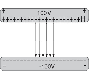
Figure 17.5 A guess as to how charge may rearrange itself on finite conducting plates.
2. For the next version of this problem, assume that the plates are composed of a line of dielectric material with uniform charge densities ρ on the top and - ρ on the bottom. Solve Poisson’s equation (17.3) in the region including the plates, and Laplace’s equation elsewhere. Experiment until you find a numerical value for ρ that gives a potential similar to that shown in Figure 17.6 for plates with fixed voltages.
3. For the final version of this problem investigate how the charges on a capacitor with finite-thickness conducting plates (Figure 17.5) distribute themselves. Since the plates are conductors, they are still equipotential surfaces at 100 and -100 V, only now they have a thickness of at least 2Δ (so we can see the difference between the potential near the top and the bottom surfaces of the plates). Such being the case, we solve Laplace’s equation (17.4) much as before to determine U(x, y). Once we have U(x, y), we substitute it into Poisson’s equation (17.3) and determine how the charge density distributes itself along the top and bottom surfaces of the plates. Hint: Since the electric field is no longer uniform, we know that the charge distribution also will no longer be uniform. In addition, since the electric field now extends beyond the ends of the capacitor and since field lines begin and end on charge, some charge may end up on the edges and outer surfaces of the plates (Figure 17.4).
4. The numerical solution to our PDE can be applied to arbitrary boundary conditions. Two boundary conditions to explore are triangular and sinusoidal:

5. Square conductors: You have designed a piece of equipment consisting of a small metal box at 100V within a larger grounded one (Figure 17.8). You find that sparking occurs between the boxes, which means that the electric field is too large. You need to determine where the field is greatest so that you can change the geometry and eliminate the sparking. Modify the program to satisfy these boundary conditions and to determine the field between the boxes. Gauss’s law tells us that the field vanishes within the inner box because it contains no charge. Plot the potential and equipotential surfaces and sketch in the electric field lines. Deduce where the electric field is most intense and try redesigning the equipment to reduce the field.
6. Cracked cylindrical capacitor: You have designed the cylindrical capacitor containing along outer cylinder surrounding a thin inner cylinder (Figure17.8 right). The cylinders have a small crack in them in order to connect them to the battery that maintains the inner cylinder at -100V and outer cylinder at 100V. Determine how this small crack affects the field configuration. In order for a unique solution to exist for this problem, place both cylinders within a large grounded box. Note that since our algorithm is based on expansion of the Laplacian in rectangular coordinates, you cannot just convert it to a radial and angle grid.
17.7 Implementation and Assessment
1. Write or modify the CD (available online: http://press.princeton.edu/landau_survey/) program to find the electric potential for a capacitor within a grounded box. Use the labeling scheme on the left in Figure 17.4.
2. To start, have your program undertake 1000 iterations and then quit. During debugging, examine how the potential changes in some key locations as you iterate toward a solution.

Figure 17.6 Left: A Gnuplot visualization of the computed electric potential for a capacitor with finite width plates. Right: An OpenDX visualization of the charge distribution along one plate determined by evaluating ∇2V(x, y) (courtesy of J. Wetzel). Note the “lightening rod” effect of charge accumulating at corners and points.
3. Repeat the process for different step sizes Δ and draw conclusions regarding the stability and accuracy of the solution.
4. Once your program produces reasonable solutions, modify it so that it stops iterating after convergence is reached, or if the number of iterations becomes too large. Rather than trying to discern small changes in highly compressed surface plots, use a numerical measure of precision, for example,

which samples the solution along the diagonal. Remember, this is a simple algorithm and so may require many iterations for high precision. You should be able to obtain changes in the trace that are less than 1 part in 104. (The break command or a while loop is useful for this type of test.)
5. Equation (17.31) expresses the successive overrelaxation technique in which convergence is accelerated by using a judicious choice of ω. Determine by trial and error the approximate best value of ω. You will be able to double the speed.
6. Now that the code is accurate, modify it to simulate a more realistic capacitor in which the plate separation is approximately 1/10 of the plate length. You should find the field more condensed and more uniform between the plates.
7. If you are working with the wire-in-the-box problem, compare your numerical solution to the analytic one (17.18). Do not be surprised if you need to sum thousands of terms before the analytic solution converges!
![]()
17.8 Electric Field Visualization (Exploration)
![]()
Plot the equipotential surfaces on a separate 2-D plot. Start with a crude, hand-drawn sketch of the electric field by drawing curves orthogonal to the equipotential lines, beginning and ending on the boundaries (where the charges lie). The regions of high density are regions of high electric field. Physics tells us that the electric field E is the negative gradient of the potential:

where ![]() is a unit vector in the i direction. While at first it may seem that some work is involved in determining these derivatives, once you have a solution for U(x, y) on a grid, it is simple to use the central-difference approximation for the derivative to determine the field, for example:
is a unit vector in the i direction. While at first it may seem that some work is involved in determining these derivatives, once you have a solution for U(x, y) on a grid, it is simple to use the central-difference approximation for the derivative to determine the field, for example:

Once you have a data file representing such a vector field, it can be visualized by plotting arrows of varying lengths and directions, or with just lines (Figure 17.7). This is possible in Maple and Mathematica [L 05] or with vectors style in Gnuplot2 where N is a normalization factor.
17.9 Laplace Quiz
You are given a simple Laplace-type equation

where x and y are Cartesian spatial coordinates and ρ(x, y) is the charge density in space.
1. Develop a simple algorithm that will permit you to solve for the potential u between two square conductors kept at fixed u, with a charge density ρ between them.
2. Make a simple sketch that shows with arrows how your algorithm works.
3. Make sure to specify how you start and terminate the algorithm.

Figure 17.7 Left: Computed equipotential surfaces and electric field lines for a realistic capacitor. Right: Equipotential surfaces and electric field lines mapped onto the surface for a 3-D capacitor constructed from two tori (see OpenDX in Appendix C).

Figure 17.8 Left: The geometry of a capacitor formed by placing two long, square cylinders within each other. Right: The geometry of a capacitor formed by placing two long, circular cylinders within each other. The cylinders are cracked on the side so that wires can enter the region.
4. Thinking outside the box![]() : Find the electric potential for all points outside the charge-free square shown in Figure 17.1. Is your solution unique?
: Find the electric potential for all points outside the charge-free square shown in Figure 17.1. Is your solution unique?
![]()
17.10 Unit II. Finite-Element Method 
In this unit we solve a simpler problem than the one in Unit I (1-D rather than 2-D), but we do it with a less simple algorithm (finite element). Our usual approach to PDEs in this text uses finite differences to approximate various derivatives in terms of the finite differences of a function evaluated upon a fixed grid. The finite-element method (FEM), in contrast, breaks space up into multiple geometric objects (elements), determines an approximate form for the solution appropriate to each element, and then matches the solutions up at the domain edges.

Figure 17.9 Two metal plates with a charge density between them. The dots are the nodes xi, and the lines connecting the nodes are the finite elements.
The theory and practice of FEM as a numerical method for solving partial differential equations have been developed over the last 30 years and still provide an active field of research. One of the theoretical strengths of FEM is that its mathematical foundations allow for elegant proofs of the convergence of solutions to many delicate problems. One of the practical strengths of FEM is that it offers great flexibility for problems on irregular domains or highly varying coefficients or singularities. Although finite differences are simpler to implement than FEM, they are less robust mathematically and less efficientin terms of computer time for big problems. Finite elementsinturn are more complicated toimplement but more appropriate and precise for complicated equations and complicated geometries. In addition, the same basic finite-element technique can be applied to many problems with only minor modifications and yields solutions that maybeevaluated for any value ofx, not just those on a grid. In fact, the finite-elements method with various preprogrammed multigrid packages has very much become the standard for large-scale practical applications. Our discussion is based upon [Shaw 92, Li, Otto].
17.11 Electric Field from Charge Density (Problem)
You are given two conducting plates a distance b-a apart, with the lower one kept at potential Ua, the upper plate at potential Ub, and a uniform charge density ρ(x) placed between them (Figure 17.9). Your problem is to compute the electric potential between the plates.
17.12 Analytic Solution
The relation between charge density ρ(x) and potential U(x) is given by Poisson’s equation (17.5). For our problem, the potential U changes only in the x direction, and so the PDE becomes the ODE:

where we have set ρ(x) = 1/4π to simplify the programming. The solution we want is subject to the Dirichlet boundary conditions:

Although we know the analytic solution, we shall develop the finite-element method for solving the ODE as if it were a PDE (it would be in 2-D) and as if we did not know the solution. Although we will not demonstrate it, this method works equally well for any charge density ρ(x).
17.13 Finite-Element (Not Difference) Methods
In afinite-element method, the domain inwhich the PDEissolved is split intofinite subdomains, called elements, and a trial solution to the PDE in each subdomain is hypothesized. Then the parameters of the trial solution are adjusted to obtain a best fit (in the sense of Chapter 8, “Solving Systems of Equations with Matrices; Data Fitting”) to the exact solution. The numerically intensive work is in finding the best values for these parameters and in matching the trial solutions for the different subdomains. A FEM solution follows six basic steps [Li]:
1. Derivation of a weak form of the PDE. This is equivalent to a least-squares minimization of the integral of the difference between the approximate and exact solutions.
2. Discretization of the computational domains.
3. Generation of interpolating or trial functions.
4. Assembly of the stiffness matrix and load vector.
5. Implementation of the boundary conditions.
6. Solution of the resulting linear system of equations.
17.13.1 Weak Form of PDE
Finite-difference methods look for an approximate solution of an approximate PDE. Finite-element methods strive to obtain the best possible global agreement of an approximate trial solution with the exact solution. We start with the differential equation

A measure of overall agreement must involve the solution U(x) over some region of space, such as the integral of the trial solution. We can obtain such a measure by converting the differential equation (17.38) to its equivalent integral or weak form. We assume that we have an approximate or trial solution Φ(x) that vanishes at the endpoints, Φ(a) = Φ(b) = 0 (we satisfy the boundary conditions later). We next multiply both sides of the differential equation (17.38) by Φ:

Next we integrate (17.39) by parts from a to b:

Equation (17.41) is the weak form of the PDE. The unknown exact solution U(x) and the trial function Φ are still to be specified. Because the approximate and exact solutions are related by the integral of their difference over the entire domain, the solution provides a global best fit to the exact solution.
17.13.2 Galerkin Spectral Decomposition
The approximate solution to a weak PDE is found via a stepwise procedure. We split the full domain of the PDE into subdomains called elements, find approximate solutions within each element, and then match the elemental solutions onto each other. For our 1-D problem the subdomain elements are straight lines of equal length, while for a 2-D problem, the elements can be parallelograms or triangles (Figure 17.9). Although life is simpler if all the finite elements are the same size, this is not necessary. Indeed, higher precision and faster run times may be obtained by picking small domains in regions where the solution is known to vary rapidly, and picking large domains in regions of slow variation.

Figure 17.10 Left: A set of overlapping basis functions φi. Each function is a triangle from xi-1 to xi+1. Middle: A Piecewise-linear function. Right: A piecewise-quadratic function.
The critical step in the finite-element method is expansion of the trial solution U in terms of a set of basis functions φi:

We chose φi’s that are convenient to compute with and then determine the unknown expansion coefficients αj. Even if the basis functions are not sines or cosines, this expansion is still called a spectral decomposition. In order to satisfy the boundary conditions, we will later add another term to the expansion. Considerable study has gone into the effectiveness of different basis functions. If the sizes of the finite elements are made sufficiently small, then good accuracy is obtained with simple piecewise-continuous basis functions, such as the triangles in Figure 17.10. Specifically, we use basis functions φi that form a triangle or “hat” between xi-1 and xi+1 and equal 1 at xi:
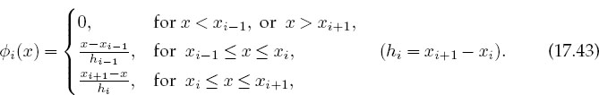
Because we have chosen φi(xi) = 1,the values of the expansion coefficients αi equal the values of the (still-to-be-determined) solution at the nodes:

Consequently, you can think of the hat functions as linear interpolations between the solution at the nodes.
17.13.2.1 SOLUTION VIA LINEAR EQUATIONS
Because the basis functions φi in (17.42) are known, solving for U(x) involves determining the coefficients αj, which are just the unknown values of U(x) on the nodes. We determine those values by substituting the expansions for U(x) and Φ(x) into the weak form of the PDE (17.41) and thereby convert them to a set of simultaneous linear equations (in the standard matrix form):
We substitute the expansion U(x) ![]() Σj=0 αjφj(x) into the weak form (17.41):
Σj=0 αjφj(x) into the weak form (17.41):

By successively selecting Φ(x) = φ0, φ1,…, φN-1, we obtain N simultaneous linear equations for the unknown αj’s:

We factor out the unknown αj’s and write out the equations explicitly:

Because we have chosen the φi’s to be the simple hat functions, the derivatives are easy to evaluate analytically (otherwise they can be done numerically):

The integrals to evaluate are

We rewrite these equations in the standard matrix form (17.46) with y constructed from the unknown αj’s, and the tridiagonal stiffness matrix A constructed from the integrals over the derivatives:

The elements in A are just combinations of inverse step sizes and so do not change for different charge densities ρ(x). The elements in b do change for different ρ’s, but the required integrals can be performed analytically or with Gaussian quadrature (Chapter 6, “Integration”). Once A and b are computed, the matrix equations are solved for the expansion coefficients αj contained in y.
17.13.2.2 DIRICHLET BOUNDARY CONDITIONS
Because the basis functions vanish at the endpoints, a solution expanded in them also vanishes there. This will not do in general, and so weadd the particular solution Uaφ0(x), which satisfies the boundary conditions [Li]:

where Ua = U(xa). We substitute U(x)-Uaφ0(x) into the weak form to obtain (N +1) simultaneous equations, still of the form Ay = b but now with

This is equivalent to adding a new element and changing the load vector:
![]()
To impose the boundary condition at x = b, we again add a term and substitute into the weak form to obtain
![]()
We now solve the linear equations Ay = b’. For 1-D problems, 100-1000 equations are common, while for 3-D problems there may be millions. Because the number of calculations varies approximately as N2, it is important to employ an efficient and accurate algorithm because round-off error can easily accumulate after thousands of steps. We recommend one from a scientific subroutine library (see Chapter 8, “Solving Systems of Equations with Matrices; Data Fitting”).
17.14 FEM Implementation and Exercises
In Listing 17.2 we give our program LaplaceFEM.java that determines the FEM solution, and in Figure 17.11 we show that solution. We see on the left that three elements do not provide good agreement with the analytic result, whereas N = 11 elements produces excellent agreement.
1. Examine the FEM solution for the choice of parameters
![]()
2. Generate your own triangulation by assigning explicit x values at the nodes over the interval [0,1].
3. Start with N = 3 and solve the equations for N values up to 1000.
4. Examine the stiffness matrix A and ensure that it is triangular.
5. Verify that the integrations used to compute the load vector b are accurate.
6. Verify that the solution of the linear equation Ay = b is correct.
7. Plot the numerical solution for U(x) for N = 10,100, and 1000 and compare with the analytic solution.

Figure 17.11 Exact (line) versus FEM solution (points) for the two-plate problem for N = 3 and N = 11 finite elements.
8. The log of the relative global error (number of significant figures) is
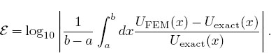
Plot the global error versus x for N = 10, 100, and 1000.
![]()


Listing 17.2 LaplaceFEM.java provides a finite-element method solution of the 1-D Laplace equation via a Galerkin spectral decomposition. The resulting matrix equations are solved with Jama. Although the algorithm is more involved than the solution via relaxation (Listing 17.1), it is a direct solution with no iteration required.
17.15 Exploration
1. Modify your program to use piecewise-quadratic functions for interpolation and compare to the linear function results.

Figure 17.12 A metallic bar insulated along its length with its ends in contact with ice.
2. Explore the resulting electric field if the charge distribution between the plates has the explicit x dependences

17.16 Unit III. Heat Flow via Time-Stepping (Leapfrogging)
Problem: You are given an aluminum bar of length L = 1 m and width w aligned along the x axis (Figure 17.12). It is insulated along its length but not at its ends. Initially the bar is at a uniform temperature of 100 K, and then both ends are placed in contact with ice water at 0K. Heat flows out of the noninsulated ends only. Your problem is to determine how the temperature will vary as we move along the length of the bar at later times.
17.17 The Parabolic Heat Equation (Theory)
A basic fact of nature is that heat flows from hot to cold, that is, from regions of high temperature to regions of low temperature. We give these words mathematical expression by stating that the rate of heat flow H through a material is proportional to the gradient of the temperature T across the material:
![]()
where K is the thermal conductivity of the material. The total amount of heat Q(t) in the material at any one time is proportional to the integral of the temperature over the material’s volume:

where C is the specific heat of the material and ρ is its density. Because energy is conserved, the rate of decrease in Q with time must equal the amount of heat flowing out of the material. After this energy balance is struck and the divergence theorem applied, the heat equation results:

The heat equation (17.57)is aparabolic PDE with space and timeas independent variables. The specification of this problem implies that there is no temperature variation in directions perpendicular to the bar (y and z), and so we have only one spatial coordinate in the Laplacian:

As given, the initial temperature of the bar and the boundary conditions are
![]()
17.17.1 Solution: Analytic Expansion
Analogous to Laplace’s equation, the analytic solution starts with the assumption that the solution separates into the product of functions of space and time:
![]()
When (17.60) is substituted into the heat equation (17.58) and the resulting equation is divided by X(x)T (t), two noncoupled ODEs result:

where k is a constant still to be determined. The boundary condition that the temperature equals zero at x = 0 requires a sine function for X:
![]()
The boundary condition that the temperature equals zero at x = L requires the sine function to vanish there:
![]()
The time function is a decaying exponential with k in the exponent:
![]()
where n can be any integer and An is an arbitrary constant. Since (17.58) is a linear equation, the most general solution is a linear superposition of all values of n:

The coefficients An are determined by the initial condition that at time t = 0 the entire bar has temperature T = 100 K:

Projecting the sine functions determines An = 4T0/nπ for n odd, and so

17.17.2 Solution: Time-Stepping
As we did with Laplace’s equation, the numerical solution is based on converting the differential equation to a finite-difference (“difference”) equation. We discretize space and time on a lattice (Figure 17.13) and solve for solutions on the lattice sites. The horizontal nodes with white centers correspond to the known values of the temperature for the initial time, while the vertical white nodes correspond to the fixed temperature along the boundaries. If we also knew the temperature for times along the bottom row, then we could use a relaxation algorithm as we did for Laplace’s equation. However, with only the top row known, we shall end up with an algorithm that steps forward in time one row at a time, as in the children’s game leapfrog.
As is often the case with PDEs, the algorithm is customized for the equation being solved and for the constraints imposed by the particular set of initial and boundary conditions. With only one row of times to start with, we use a forward-difference approximation for the time derivative of the temperature:
Because we know the spatial variation of the temperature along the entire top row and the left and right sides, we are less constrained with the space derivative as with the time derivative. Consequently, as we did with the Laplace equation, we use the more accurate central-difference approximation for the space derivative:


Figure 17.13 The algorithm for the heat equation in which the temperature at the location x= i Δxand time t= (j+1)Δt is computed from the temperature values at three points of an earlier time. The nodes with white centers correspond to known initial and boundary conditions. (The boundaries are placed artificially close for illustrative purposes.)
Substitution of these approximations into (17.58) yields the heat difference equation

We reorder (17.70) into a form in which T can be stepped forward in t:

where x = iΔx and t = jΔt. This algorithm is explicit because it provides a solution in terms of known values of the temperature. If we tried to solve for the temperature at all lattice sites in Figure. 17.13 simultaneously, then we would have an implicit algorithm that requires us to solve equations involving unknown values of the temperature. We see that the temperature at space-time point (i,j +1) is computed from the three temperature values at an earlier time j and at adjacent space values i ± 1,i. We start the solution at the top row, moving it forward in time for as long as we want and keeping the temperature along the ends fixed at 0 K (Figure 17.14).

Figure 17.14 A numerical calculation of the temperature versus position and versus time, with isotherm contours projected onto the horizontal plane on the left and with a red-blue color scale used to indicate temperature on the right (the color is visible on the figures on the CD (available online: http://press.princeton.edu/landau_survey/)).
17.17.3 Von Neumann Stability Assessment
When we solve a PDE by converting it to a difference equation, we hope that the solution of the latter is a good approximation to the solution of the former. If the difference-equation solution diverges, then we know we have a bad approximation, but if it converges, then we may feel confident that we have a good approximation to the PDE. The von Neumann stability analysis is based on the assumption that eigenmodes of the difference equation can be written as
where x = m Δx and t = jΔt, but ![]() is the imaginary number. The constant k in (17.72) is an unknown wave vector (2π/λ), and ξ(k) is an unknown complex function. View (17.72) as a basis function that oscillates in space (the exponential) with an amplitude or amplification factor ξ(k) j that increases by a power of ξ for each time step. If the general solution to the difference equation can be expanded in terms of these eigenmodes, then the general solution will be stable if the eigenmodes are stable. Clearly, for an eigenmode to be stable, the amplitude ξ cannot grow in time j, which means |ξ(k) | < 1 for all values of the parameter k [Pres 94, Anc 02].
is the imaginary number. The constant k in (17.72) is an unknown wave vector (2π/λ), and ξ(k) is an unknown complex function. View (17.72) as a basis function that oscillates in space (the exponential) with an amplitude or amplification factor ξ(k) j that increases by a power of ξ for each time step. If the general solution to the difference equation can be expanded in terms of these eigenmodes, then the general solution will be stable if the eigenmodes are stable. Clearly, for an eigenmode to be stable, the amplitude ξ cannot grow in time j, which means |ξ(k) | < 1 for all values of the parameter k [Pres 94, Anc 02].
Application of a stability analysis is more straightforward than it might appear. We just substitute the expression (17.72) into the difference equation (17.71):

After canceling some common factors, it is easy to solve for ξ:
![]()
In order for |ξ(k)| < 1 for all possible k values, we must have

This equation tells us that if we make the time step Δt smaller, we will always improve the stability, as we would expect. But if we decrease the space step Δx without a simultaneous quadratic increase in the time step, we will worsen the stability. The lack of space-time symmetry arises from our use of stepping in time but not in space.
In general, you should perform a stability analysis for every PDE you have to solve, although it can get complicated [Pres 94]. Yet even if you do not, the lesson here is that you may have to try different combinations of Δx and Δt variations until a stable, reasonable solution is obtained. You may expect, nonetheless, that there are choices for Δx and Δt for which the numerical solution fails and that simply decreasing an individual Δx or Δt, in the hope that this will increase precision, may not improve the solution.

Listing 17.3 EqHeat.java solves the heat equation for a 1-D space and time by leapfrogging (time-stepping) the initial conditions forward in time. You will need to adjust the parameters to obtain a solution like those in the figures.
17.17.4 Heat Equation Implementation
Recollect that we want to solve for the temperature distribution within an aluminum bar of length L = 1 m subject to the boundary and initial conditions
The thermal conductivity, specific heat, and density for Al are
![]()
1. Write or modify EqHeat.java in Listing 17.3 to solve the heat equation.
2. Define a 2-D array T[101][2] for the temperature as a function of space and time. The first index is for the 100 space divisions of the bar, and the second index is for present and past times (because you may have to make thousands of time steps, you save memory by saving only two times).
3. For time t = 0 (j = 1), initialize T so that all points on the bar except the ends are at 100 K. Set the temperatures of the ends to 0K.
4. Apply (17.68) to obtain the temperature at the next time step.
5. Assign the present-time values of the temperature to the past values:
T[i][1] = T[i][2], i = 1,.. ., 101.
6. Start with 50 time steps. Once you are confident the program is running properly, use thousands of steps to see the bar cool smoothly with time. For approximately every 500 time steps, print the time and temperature along the bar.
17.18 Assessment and Visualization
1. Check that your program gives a temperature distribution that varies smoothly along the bar and agrees with the boundary conditions, as in Figure 17.14.
2. Check that your program gives a temperature distribution that varies smoothly with time and attains equilibrium. You may have to vary the time and space steps to obtain well-behaved solutions.
3. Compare the analytic and numeric solutions (and the wall times needed to compute them). If the solutions differ, suspect the one that does not appear smooth and continuous.
4. Make surface plots of temperature versus position for several times.
5. Better yet, make a surface plot of temperature versus position versus time.
6. Plot the isotherms (contours of constant temperature).
7. Stability test: Check (17.74) that the temperature diverges in t if η > ¼.
8. Material dependence: Repeat the calculation for iron. Note that the stability condition requires you to change the size of the time step.

Figure 17.15 Temperature versus position and time when two bars at differing temperatures are placed in contact at t = 0. The projected contours show the isotherms.
9. Initial sinusoidal distribution sin(πx/L): Compare to the analytic solution,
10. Two bars in contact: Two identical bars 0.25m long are placed in contact along one of their ends with their other ends kept at 0K. One is kept in a heat bath at 100K, and the other at 50 K. Determine how the temperature varies with time and location (Figure 17.15).
11. Radiating bar (Newton’s cooling): Imagine now that instead of being insulated along its length, a bar is in contact with an environment at a temperature Te. Newton’s law of cooling (radiation) says that the rate of temperature change due to radiation is

where h is a positive constant. This leads to the modified heat equation

Modify the algorithm to include Newton’s cooling and compare the cooling of this bar with that of the insulated bar.
![]()
17.19 Improved Heat Flow: Crank-Nicolson Method
The Crank-Nicolson method [C&N 47] provides a higher degree of precision for the heat equation (17.57). This method calculates the time derivative with a central-difference approximation, in contrast to the forward-difference approximation used previously. In order to avoid introducing error for the initial time step, where only a single time value is known, the method uses a split time step,3 so that time is advanced from time t to t + Δt/2:

Yes, we know that this looks just like the forward-difference approximation for the derivative at time t +Δt, for which it would be a bad approximation; regardless, it is a better approximation for the derivative at time t + Δt/2, though it makes the computation more complicated. Likewise, in (17.68) we gave the central-difference approximation for the second space derivative for time t. For t = t + Δt/2, that becomes

In terms of these expressions, the heat difference equation is

We group together terms involving the same temperature to obtain an equation with future times on the LHS and present times on the RHS:

This equation represents an implicit scheme for the temperature Ti,j, where the word“implicit” meansthatwemustsolve simultaneousequationstoobtain the full solution for all space. Incontrast, an explicit scheme requires iterationto arriveatthe solution.Itis possibleto solve (17.82) simultaneously for all unknown temperatures (1 ≤ i ≤ N) at times j and j +1. We start with the initial temperature distribution throughout all of space, the boundary conditions at the ends of the bar for all times, and the approximate values from the first derivative:

We rearrange (17.82) so that we can use these known values of T to step the j = 0 solution forward in time by expressing (17.82) as a set of simultaneous linear equations (in matrix form):

Observe that the T’s on the RHS are all at the present time j for various positions, and at future time j +1 for the two ends (whose Ts are known for all times via the boundary conditions). We start the algorithm with the Ti,j=0 values of the initial conditions, then solve a matrix equation to obtain Ti,j=1. With that we know all the terms on the RHS of the equations (j = 1 throughout the bar and j = 2 at the ends) and so can repeat the solution of the matrix equations to obtain the temperature throughout the bar for j = 2. So again we time-step forward, only now we solve matrix equations at each step. That gives us the spatial solution directly.
Not only is the Crank-Nicolson method more precise than the low-order time-stepping method of Unit III, but it also is stable for all values of Δt and Δx. To prove that, we apply the von Neumann stability analysis discussed in §17.17.3 to the Crank-Nicolson algorithm by substituting (17.71) into (17.82). This determines an amplification factor

Because sin2() is positive-definite, this proves that ξ ≤ 1 for all Δt, Δx, and k.
17.19.1 Solution of Tridiagonal Matrix Equations
The Crank-Nicolson equations (17.83) are in the standard [A]x = b form for linear equations, and so we can use our previous methods to solve them. Nonetheless, because the coefficient matrix [A] is tridiagonal (zero elements except for the main diagonal and two diagonals on either side of it),

a more robust and faster solution exists that makes this implicit method as fast as an explicit one. Because tridiagonal systems occur frequently, we now outline the specialized technique for solving them [Pres 94]. If we store the matrix elements ai,j using both subscripts, then we will need N2 locations for elements and N2 operations to access them. However, for a tridiagonal matrix, we need to store only the vectors {di}i=1 N, {ci}i=1 N, and {ai}i=1 N, along, above, and below the diagonals. The single subscripts on ai, di, and ci reduce the processing from N2 to (3N — 2) elements.
We solve the matrix equation by manipulating the individual equations until the coefficient matrix is upper triangular with all the elements of the main diagonal equal to 1. We start by dividing the first equation by d1, then subtract a2 times the first equation,

and then dividing the second equation by the second diagonal element,

Assuming that we can repeat these steps without ever dividing by zero, the system of equations will be reduced to upper triangular form,

where h1 = c1/d1 and p1 = b1/d1. We then recur for the others elements:

Finally, back substitution leads to the explicit solution for the unknowns:
![]()
In Listing 17.4 we give the program HeatCNTridiag.java that solves the heat equation using the Crank–Nicolson algorithm via a triadiagonal reduction.

Listing 17.4 HeatCNTridiag.java is the complete program for solution of the heat equation in one space dimension and time via the Crank–Nicolson method. The resulting matrix equations are solved via a technique specialized to tridiagonal matrices.
17.19.2 Crank–Nicolson Method Implementation and Assessment
Use the Crank–Nicolson method to solve for the heat flow in the metal bar in §17.16.
1. Write a program using the Crank–Nicolson method to solve the heat equation for at least 100 time steps.
2. Solve the linear system of equations (17.83) using either JAMA or the special tridiagonal algorithm.
3. Check the stability of your solution by choosing different values for the time and space steps.
4. Construct a contoured surface plot of temperature versus position and versus time.
5. Compare the implicit and explicit algorithms used in this chapter for relative precision and speed. You may assume that a stable answer that uses very small time steps is accurate.
1 Although conclusions drawn for exact PDEs may differ from those drawn for the finite-difference equations, they are usually the same; in fact, Morse and Feshbach [M&F 53] use the finite-difference form to derive the relations between boundary conditions and uniqueness for each type of equation shown in Table 17.1 [Jack 88].
2 The Gnuplot command plot “Laplace_field.dat” using 1:2:3:4 with Vectors plots variable-length arrows at (x, y) with components Dx ex Ex and Dy ex Ey. You determine empirically what scale factor gives you the best visualization (nonoverlapping arrows). Accordingly you output data lines of the form (x, y, Ex/N, Ey/N)
3 In §18.6.1wedevelop another split-time algorithm for solution of the Schrödinger equation, where the real and imaginary parts of the wave function are computed at times that differ by Δt/2.