
18
PDE Waves: String, Quantum Packet, and E&M
In this chapter we explore the numerical solution of a number of PDEs known as wave equations . We have two purposes in mind. First, especially if you have skipped the discussion of the heat equation in Chapter 17, “PDES for Electrostatics & Heat Flow,” we wish to give another example of how initial conditions in time are treated with a time-stepping or leapfrog algorithm. Second, we wish to demonstrate that once we have a working algorithm for solving a wave equation, we can include considerably more physics than is possible with analytic treatments. Unit I deals with a number of aspects of waves on a string. Unit II deals with quantum wave packets, which have their real and imaginary parts solved for at different (split) times. Unit III extends the treatment to electromagnetic waves that have the extra complication of being vector waves with interconnected E and H fields. Shallow-water waves, dispersion, and shock waves are studied in Chapter 19, “Solitons and Computational Fluid Dynamics.”
18.1 Unit I. Vibrating String
Problem: Recall the demonstration from elementary physics in which a string tied down at both ends is plucked “gently” at one location and a pulse is observed to travel along the string. Likewise, if the string has one end free and you shake it just right, a standing-wave pattern is set up in which the nodes remain in place and the antinodes move just up and down. Your problem is to develop an accurate model for wave propagation on a string and to see if you can set up traveling- and standing-wave patterns.1
18.2 The Hyperbolic Wave Equation (Theory)
Consider a string of length L tied down at both ends (Figure 18.1 left). The string has a constant density ρ per unit length, a constant tension T, is subject to no frictional forces, and the tension is high enough that we may ignore sagging due to gravity. We assume that the displacement of the string y(x, t) from its rest position is in the vertical direction only and that it is a function of the horizontal location along the string x and the time t.

Figure 18.1 Left:A stretched string of length L tied down at both ends and under high enough tension to ignore gravity. The vertical disturbance of the string from its equilibrium position is y(x, t). Right: A differential element of the string showing how the string’s displacement leads to the restoring force.
To obtain a simple linear equation of motion (nonlinear wave equations are discussed in Chapter 19, “Solitons & Computational Fluid Dynamics”), we assume that the string’s relative displacement y(x,t)/L and slope ∂y/∂x are small. We isolate an infinitesimal section Δx of the string (Figure 18.1 right) and see that the difference in the vertical components of the tension at either end of the string produces the restoring force that accelerates this section of the string in the vertical direction. By applying Newton’s laws to this section, we obtain the familiar wave equation:

where we have assumed that θ is small enough for sin θ ![]() tan θ = ∂y/∂x. The existence of two independent variables x and t makes this a PDE. The constant c is the velocity with which a disturbance travels along the wave and is seen to decrease for a heavier string and increase for a tighter one. Note that this signal velocity c is not the same as the velocity of a string element ∂y/∂t.
tan θ = ∂y/∂x. The existence of two independent variables x and t makes this a PDE. The constant c is the velocity with which a disturbance travels along the wave and is seen to decrease for a heavier string and increase for a tighter one. Note that this signal velocity c is not the same as the velocity of a string element ∂y/∂t.
The initial condition for our problem is that the string is plucked gently and released. We assume that the “pluck” places the string in a triangular shape with the center of triangle ![]() of the way down the string and with a height of 1:
of the way down the string and with a height of 1:

Because (18.2) is second-order in time, a second initial condition (beyond initial displacement) is needed to determine the solution. We interpret the “gentleness” of the pluck to mean the string is released from rest:
The boundary conditions have both ends of the string tied down for all times:
![]()
18.2.1 Solution via Normal-Mode Expansion
The analytic solution to (18.2) is obtained via the familiar separation-of-variables technique. We assume that the solution is the product of a function of space and a function of time:
![]()
We substitute (18.6) into (18.2), divide by y(x, t), and are left with an equation that has a solution only if there are solutions to the two ODEs:

The angular frequency ω and the wave vector k are determined by demanding that the solutions satisfy the boundary conditions. Specifically, the string being attached at both ends demands

where the frequency of this nth normal mode is also fixed. In fact, it is the single frequency of oscillation that defines a normal mode. The initial condition (18.3) of zero velocity, ∂y/∂t(t = 0) = 0, requires the Cn values in (18.10) to be zero. Putting the pieces together, the normal-mode solutions are
![]()
Since the wave equation (18.2) is linear in y, the principle of linear superposition holds and the most general solution for waves on a string with fixed ends can be
written as the sum of normal modes:

(Yet we will lose linear superposition once we include nonlinear terms in the wave equation.) The Fourier coefficient Bn is determined by the second initial condition (18.3), which describes how the wave is plucked:

Multiply both sides by sin mk0x, substitute the value of y(x, 0) from (18.3), and integrate from 0 to l to obtain
![]()
You will be asked to compare the Fourier series (18.12) to our numerical solution. While it is in the nature of the approximation that the precision of the numerical solution depends on the choice of step sizes, it is also revealing to realize that the precision of the analytic solution depends on summing an infinite number of terms, which can be done only approximately.
18.2.2 Algorithm: Time-Stepping
As with Laplace’s equation and the heat equation, we look for a solution y(x, t) only for discrete values of the independent variables x and t on a grid (Figure 18.2):

In contrast to Laplace’s equation where the grid was in two space dimensions, the grid in Figure 18.2 is in both space and time. That being the case, moving across a row corresponds to increasing x values along the string for a fixed time, while moving down a column corresponds to increasing time steps for a fixed position. Even though the grid in Figure 18.2 may be square, we cannot use a relaxation technique for the solution because we do not know the solution on all four sides. The boundary conditions determine the solution along the right and left sides, while the initial time condition determines the solution along the top.
As with the Laplace equation, we use the central-difference approximation to discretize the wave equation into a difference equation. First we express the second derivatives in terms of finite differences:


Figure 18.2 The solutions of the wave equation for four earlier space-time points are used to obtain the solution at the present time. The boundary and initial conditions are indicated by the white-centered dots.
Substituting (18.17) in the wave equation (18.2) yields the difference equation
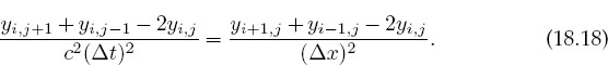
Notice that this equation contains three time values: j+1 = the future, j = the present, and j-1 = the past. Consequently, we rearrange it into a form that permits us to predict the future solution from the present and past solutions:

Here c’ is a combination of numerical parameters with the dimension of velocity whose size relative to c determines the stability of the algorithm. The algorithm (18.19) propagates the wave from the two earlier times, j and j — 1, and from three nearby positions, i — 1, i, and i + 1, to a later time j + 1 and a single space position i (Figure 18.2).
As you have seen in our discussion of the heat equation, a leapfrog method is quite different from a relaxation technique. We start with the solution along the topmost row and then move down one step at a time. If we write the solution for present times to a file, then we need to store only three time values on the computer, which saves memory. In fact, because the time steps must be quite small to obtain high precision, you may want to store the solution only for every fifth or tenth time.
Initializing the recurrence relation is a bit tricky because it requires displacements from two earlier times, whereas the initial conditions are for only one time. Nonetheless, the rest condition (18.3) when combined with the forward-difference approximation lets us extrapolate to negative time:

Here we take the initial time as j = 1, and so j = 0 corresponds to t = —Δt. Substituting this relation into (18.19) yields for the initial step

Equation (18.21) uses the solution throughout all space at the initial time t = 0 to propagate (leapfrog) it forward to a time Δt. Subsequent time steps use (18.19) and are continued for as long as you like.
As is also true with the heat equation, the success of the numerical method depends on the relative sizes of the time and space steps. If we apply a von Neumann stability analysis to this problem by substituting ym,j = ξj exp(ikm Δx), as we did in §17.17.3, a complicated equation results. Nonetheless, [Pres 94] shows that the difference-equation solution will be stable for the general class of transport equations if

Equation (18.22) means that the solution gets better with smaller time steps but gets worse for smaller space steps (unless you simultaneously make the time step smaller). Having different sensitivities to the time and space steps may appear surprising because the wave equation (18.2) is symmetric in x and t, yet the symmetry is broken by the nonsymmetric initial and boundary conditions.
Exercise: Figure out a procedure for solving for the wave equation for all times in just one step. Estimate how much memory would be required.
Exercise: Try to figure out a procedure for solving for the wave motion with a relaxation technique. What would you take as your initial guess, and how would you know when the procedure has converged?
![]()
18.2.3 Wave Equation Implementation
The program EqString.java in Listing 18.1 solves the wave equation for a string of length L= 1 m with its ends fixed and with the gently plucked initial conditions. Note that our use of L = 1 violates our assumption that y/L << 1 but makes it easy to display the results; you should try L = 1000 to be realistic. The values of density and tension are entered as constants, ρ = 0.01 kg/m and T = 40 N, with the space grid set at 101 points, corresponding to Δ = 0.01 cm.

Listing 18.1 EqString.java solves the wave equation via time stepping for a string of length L= 1 m with its ends fixed and with the gently plucked initial conditions. You will need to modify this code to include new physics.
18.2.4 Assessment and Exploration
1. Solve the wave equation and make a surface plot of displacement versus time and position.
2. Explore a number of space and time step combinations. In particular, try steps that satisfy and that do not satisfy the Courant condition (18.22). Does your exploration conform with the stability condition?
3. Compare the analytic and numeric solutions, summing at least 200 terms in the analytic solution.
4. Use the plotted time dependence to estimate the peak’s propagation velocity c. Compare the deduced c to (18.2).
5. Our solution of the wave equation for a plucked string leads to the formation of a wave packet that corresponds to the sum of multiple normal modes of the string. On the right in Figure 18.3 we show the motion resulting from the string initially placed in a single normal mode (standing wave),

Figure 18.3 The vertical displacement as a function of position x and time t. A string initially placed in a standing wave on a string with friction. Notice how the standing wave moves up and down with time. (Courtesy of J. Wiren.)
Modify the program to incorporate this initial condition and see if a normal mode results.
6. Observe the motion of the wave for initial conditions corresponding to the sum of two adjacent normal modes. Does beating occur?
7. When a string is plucked near its end, a pulse reflects off the ends and bounces back and forth. Change the initial conditions of the model program to one corresponding to a string plucked exactly in its middle and see if a traveling or a standing wave results.
8. ![]() Figure 18.4 shows the wave packets that result as a function of time for initial conditions corresponding to the double pluck indicated on the left in the figure. Verify that initial conditions of the form
Figure 18.4 shows the wave packets that result as a function of time for initial conditions corresponding to the double pluck indicated on the left in the figure. Verify that initial conditions of the form

lead to this type of a repeating pattern. In particular, observe whether the pulses move or just oscillate up and down.
![]()

Figure 18.4 The vertical displacement as a function of position and time of a string initially plucked simultaneously at two points, as shown by arrows. Note that the initial peaks break up into waves traveling to the right and to the left. The traveling waves invert on reflection from the fixed ends. As a consequence of these inversions, the ![]() 12 wave is an inverted t= 0 wave.
12 wave is an inverted t= 0 wave.
18.3 Waves with Friction (Extension)
The string problem we have investigated so far can be handled by either a numerical or an analytic technique. We now wish to extend the theory to include some more realistic physics. These extensions have only numerical solutions.
Real plucked strings do not vibrate forever because the real world contains friction. Consider again the element of a string between x and x+dx (Figure 18.1 right) but now imagine that this element is moving in a viscous fluid such as air. An approximate model has the frictional force pointing in a direction opposite the (vertical) velocity of the string and proportional to that velocity, as well as proportional to the length of the string element:

where κ is a constant that is proportional to the viscosity of the medium in which the string is vibrating. Including this force in the equation of motion changes the wave equation to

In Figure 18.3 we show the resulting motion of a string plucked in the middle when friction is included. Observe how the initial pluck breaks up into waves traveling to the right and to the left that are reflected and inverted by the fixed ends. Because those parts of the wave with the higher velocity experience greater friction, the peak tends to be smoothed out the most as time progresses.
Exercise: Generalize the algorithm used to solve the wave equation to now include friction and check if the wave’s behavior seems physical (damps in time). Start with T = 40 N and ρ = 10 kg/m and pick a value of κ large enough to cause a noticeable effect but not so large as to stop the oscillations. As a check, reverse the sign of κ and see if the wave grows in time (which would eventually violate our assumption of small oscillations).
![]()
18.4 Waves for Variable Tension and Density (Extension)
We have derived the propagation velocity for waves on a string as c = ![]() This says that waves move slower in regions of high density and faster in regions of high tension. If the density of the string varies, for instance, by having the ends thicker in order to support the weight of the middle, then c will no longer be a constant and our wave equation will need to be extended. In addition, if the density increases, then so will the tension because it takes greater tension to accelerate a greater mass. If gravity acts, then we will also expect the tension at the ends of the string to be higher than in the middle because the ends must support the entire weight of the string.
This says that waves move slower in regions of high density and faster in regions of high tension. If the density of the string varies, for instance, by having the ends thicker in order to support the weight of the middle, then c will no longer be a constant and our wave equation will need to be extended. In addition, if the density increases, then so will the tension because it takes greater tension to accelerate a greater mass. If gravity acts, then we will also expect the tension at the ends of the string to be higher than in the middle because the ends must support the entire weight of the string.
To derive the equation for wave motion with variable density and tension, consider again the element of a string (Figure 18.1 right) used in our derivation of the wave equation. If we do not assume the tension T is constant, then Newton’s second law gives

If ρ(x) and T(x) are known functions, then these equations can be solved with just a small modification of our algorithm.
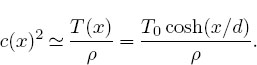
In §18.4.1 we will solve for the tension in a string due to gravity. Readers interested in an alternate easier problem that still shows the new physics may assume that the density and tension are proportional:
While we would expect the tension to be greater in regions of higher density (more mass to move and support), being proportional is clearly just an approximation. Substitution of these relations into (18.27) yields the new wave equation:

Here c is a constant that would be the wave velocity if α = 0. This equation is similar to the wave equation with friction, only now the first derivative is with respect to x and not t. The corresponding difference equation follows from using central-difference approximations for the derivatives:

18.4.1 Waves on a Catenary
Up until this point we have been ignoring the effect of gravity upon our string’s shape and tension. This is a good approximation if there is very little sag in the string, as might happen if the tension is very high and the string is light. Even if there is some sag, our solution for y(x, t) could be used as the disturbance about the equilibrium shape. However, if the string is massive, say, like a chain or heavy cable, then the sag in the middle caused by gravity could be quite large (Figure 18.5), and the resulting variation in shape and tension needs to be incorporated into the wave equation. Because the tension is no longer uniform, waves travel faster near the ends of the string, which are under greater tension since they must support the entire weight of the string.
18.4.2 Derivation of a Catenary Shape
Consider a string of uniform density ρ acted upon by gravity. To avoid confusion with our use of y(x) to describe a disturbance on a string, we call u(x) the equilibrium shape of the string (Figure 18.5). The statics problem we need to solve is to determine the shape u(x) and the tension T(x). The inset in Figure 18.5 is a free-body diagram of the midpoint of the string and shows that the weight W of this section of arc length s is balanced by the vertical component of the tension T. The horizonal tension T0 is balanced by the horizontal component of T:

Figure 18.5 Left: A uniform string suspended from its ends in a gravitational field assumes a catenary shape. Right: A force diagram of a section of the catenary at its lowest point. The tension now varies along the string.

The trick is to convert (18.32) to a differential equation that we can solve. We do that by replacing the slope tanθ by the derivative du/dx and taking the derivative with respect to x:

where D is a combination of constants with the dimension of length. Equation (18.34) is the equation for the catenary and has the solution [Becker 54]

Here we have chosen the x axis to lie a distance D below the bottom of the catenary (Figure 18.5) so that x = 0 is at the center of the string where y = D and T = T0. Equation (18.33) tells us the arc length s = Ddu/dx, so we can solve for s(x) and, via (18.31), for the tension T(x):

It is this variation in tension that causes the wave velocity to change for different positions on the string.
18.4.3 Catenary and Frictional Wave Exercises
We have given you the program EqString.java (Listing 18.1) that solves the wave equation. Modify it to produce waves on a catenary including friction or for the assumed density and tension given by (18.28) with α = 0.5, T0 = 40 N, and ρ0 = 0.01 kg/m. (The instructor’s CD (available online: http://press.princeton.edu/landau_survey/) contains the programs CatFriction.java and CatString.java that do this.)
1. Look for some interesting cases and create surface plots of the results.
2. Explain in words how the waves dampen and how a wave’s velocity appears to change. The behavior you obtain may look something like that shown in Figure 18.6.
3. Normal modes: Search for normal-mode solutions of the variable-tension wave equation, that is, solutions that vary as
![]()
Try using this form to start your program and see if you can find standing waves. Use large values for ω.
4. When conducting physics demonstrations, we set up standing-wave patterns by driving one end of the string periodically. Try doing the same with your program; that is, build into your code the condition that for all times
![]()
Try to vary A and ω until a normal mode (standing wave) is obtained.
5. (For the exponential density case.) If you were able to find standing waves, then verify that this string acts like a high-frequency filter, that is, that there is a frequency below which no waves occur.
6. For the catenary problem, plot your results showing both the disturbance u(x, t) about the catenary and the actual height y(x, t) above the horizontal for a plucked string initial condition.

Figure 18.6 The wave motion of a plucked catenary with friction. (Courtesy of Juan Vanegas.)
7. Try the first two normal modes for a uniform string as the initial conditions for the catenary. These should be close to, but not exactly, normal modes.
8. We derived the normal modes for a uniform string after assuming that k(x) = ω/c(x)is a constant.For a catenary without too much x variation in the tension, we should be able to make the approximation
See if you get a better representation of the first two normal modes if you include some x dependence in k.
![]()
18.5 Unit II. Quantum Wave Packets
Problem: An experiment places an electron with a definite momentum and position in a 1-D region of space the size of an atom. It is confined to that region by some kind of attractive potential. Your problem is to determine the resultant electron behavior in time and space.
18.6 Time-Dependent Schrödinger Equation (Theory)
Because the region of confinement is the size of an atom, we must solve this problem quantum mechanically. Nevertheless, it is different from the problem of a particle confined to a box considered in Chapter 9, “Differential Equation Applications,” because now we are starting with a particle of definite momentum and position. In Chapter 9 we had a time-independent situation in which we had to solve the eigenvalue problem. Now the definite momentum and position of the electron imply that the solution is a wave packet, which is not an eigenstate with a uniform time dependence of exp(—iωt). Consequently, we must now solve the time-dependent Schrödinger equation.
We model an electron initially localized in space at x = 5 with momentum ko (![]() = 1 in our units) by a wave function that is a wave packet consisting of a Gaussian multiplying a plane wave:
= 1 in our units) by a wave function that is a wave packet consisting of a Gaussian multiplying a plane wave:

To solve the problem we must determine the wave function for all later times. If (18.38) were an eigenstate of the Hamiltonian, its exp(−iωt) time dependence can be factored out of the Schrödinger equation (as is usually done in textbooks). However, Hψ≠Eψ for this ψ, and so we must solve the full time-dependent Schrödinger equation. To show you where we are going, the resulting wave packet behavior is shown in Figures 18.7 and 18.8.
The time and space evolution of a quantum particle is described by the 1-D time-dependent Schrödinger equation,

where we have set 2m = 1 to keep the equations simple. Because the initial wave function is complex (in order to have a definite momentum associated with it), the wave function will be complex for all times. Accordingly, we decompose the wave function into its real and imaginary parts:

where V (x) is the potential acting on the particle.

Figure 18.7 The position as a function of time of a localized electron confined to a square well (computed with the code SqWell.java available on the instructor’s CD: http://press.princeton.edu/landau_survey/). The electron is initially on the right with a Gaussian wave packet. In time, the wave packet spreads out and collides with the walls.

Figure 18.8 The probability density as a function of time for an electron confined to a 1-D harmonic oscillator potential well. On the left is a conventional surface plot from Gnuplot, while on the right is a color visualization from OpenDX.
18.6.1 Finite-Difference Algorithm
The time-dependent Schrödinger equation can be solved with both implicit (large-matrix) and explicit (leapfrog) methods. The extra challenge with the Schrödinger equation is to ensure that the integral of the probability density ![]() remains constant (conserved) to a high level of precision for all time. For our project we use an explicit method that improves the numerical conservation of probability by solving for the real and imaginary parts of the wave function at slightly different or “staggered” times [Ask 77, Viss 91, MLP 00]. Explicitly, the real part R is determined at times 0, Δt,…, and the imaginary part
remains constant (conserved) to a high level of precision for all time. For our project we use an explicit method that improves the numerical conservation of probability by solving for the real and imaginary parts of the wave function at slightly different or “staggered” times [Ask 77, Viss 91, MLP 00]. Explicitly, the real part R is determined at times 0, Δt,…, and the imaginary part ![]() The algorithm is based on (what else?) the Taylor expansions of R and I:
The algorithm is based on (what else?) the Taylor expansions of R and I:

where the superscript n indicates the time and the subscript i the position.
The probability density ρ is defined in terms of the wave function evaluated at three different times:

Although probability is not conserved exactly with this algorithm, the error is two orders higher than that in the wave function, and this is usually quite satisfactory. If it is not, then we need to use smaller steps. While this definition of ρ may seem strange, it reduces to the usual one for Δ t → 0 and so can be viewed as part of the art of numerical analysis. You will investigate just how well probability is conserved. We refer the reader to [Koon 86, Viss 91] for details on the stability of the algorithm.
18.6.2 Wave Packet Implementation and Animation
In Listing 18.2 you will find the program Harmos.java that solves for the motion of the wave packet (18.38) inside a harmonic oscillator potential. The program Slit.java on the instructor’s CD (available online: http://press.princeton.edu/landau_survey/) solves for the motion of a Gaussian wave packet as it passes through a slit (Figure 18.10). You should solve for a wave packet confined to the square well:

1. Define arrays psr[751][2] and psi[751][2] for the real and imaginary parts of ψ, and Rho[751] for the probability. The first subscript refers to the x position on the grid, and the second to the present and future times.
2. Use the values σ0 = 0.5, Δx = 0.02, ko = 17π, and Δt = 2Δx2.
3. Use equation (18.38) for the initial wave packet to define psr[j][1] for all j at t = 0 and to define psi[j][1] at t = 2Δt.
4. Set Rho[1] = Rho[751] = 0.0 because the wave function must vanish at the infinitely high well walls.
5. Increment time by ½Δt. Use (18.45) to compute psr[j][2] in terms of psr[j][1], and (18.46) to compute psi[j][2] in terms of psi[j][1].
6. Repeat the steps through all of space, that is, for i = 2-750.
7. Throughout all of space, replace the present wave packet (second index equal to 1) by the future wave packet (second index 2).
8. After you are sure that the program is running properly, repeat the time-stepping for ~5000 steps.

Listing 18.2 Harmos.java solves the time-dependent Schrödinger equation for a particle described by a Gaussian wave packet moving within a harmonic oscillator potential.
1. Animation: Output the probability density after every 200 steps for use in animation.
![]()
2. Make a surface plot of probability versus position versus time. This should look like Figure 18.7 or 18.8.
3. Make an animation showing the wave function as a function of time.
4. Check how well the probability is conserved for early and late times by determining the integral of the probability over all of space, ![]() and seeing by how much it changes in time (its specific value doesn’t matter because that’s just normalization).
and seeing by how much it changes in time (its specific value doesn’t matter because that’s just normalization).
5. What might be a good explanation of why collisions with the walls cause the wave packet to broaden and break up? (Hint: The collisions do not appear so disruptive when a Gaussian wave packet is confined within a harmonic oscillator potential well.)
![]()
18.7 Wave Packets in Other Wells (Exploration)
1-D Well: Now confine the electron to lie within the harmonic oscillator potential:

Take the momentum k0 = 3π, the space step Δx = 0.02, and the time step Δt = | Δx2. Note that the wave packet broadens yet returns to its initial shape!
2-D Well ![]() : Now confine the electron to lie within a 2-D parabolic tube (Figure 18.9):
: Now confine the electron to lie within a 2-D parabolic tube (Figure 18.9):
![]()
The extra degree of freedom means that we must solve the 2-D PDE:

Assume that the electron’s initial localization is described by the 2-D Gaussian wave packet:

Note that you can solve the 2-D equation by extending the method we just used in 1-D or you can look at the next section where we develop a special algorithm.
18.8 Algorithm for the 2-D Schrödinger Equation
One way to develop an algorithm for solving the time-dependent Schrödinger equation in 2-D is to extend the 1-D algorithm to another dimension. Rather than do that, we apply quantum theory directly to obtain a more powerful algorithm [MLP 00]. First we note that equation (18.48) can be integrated in a formal sense [L&L,M 76] to obtain the operator solution:

Figure 18.9 The probability density as a function of x and y of an electron confined to a 2-D parabolic tube. The electron’s initial localization is described by a Gaussian wave packet in both the x and y directions. The times are 100, 300, and 500 steps.

where U(t) is an operator that translates a wave function by an amount of time t and H is the Hamiltonian operator. From this formal solution we deduce that a wave packet can be translated ahead by time Δt via
![]()
where the superscripts denote time t = nΔt and the subscripts denote the two spatial variables x = iΔx and y = jΔy. Likewise, the inverse of the time evolution operator moves the solution back one time step:
![]()
While it would be nice to have an algorithm based on a direct application of (18.52), the references show that the resulting algorithm is not stable. That being so, we base our algorithm on an indirect application [Ask 77], namely, the relation between the difference in ψn+1 and ψn-1:
![]()
where the difference in sign of the exponents is to be noted. The algorithm derives from combining the O(Δx2) expression for the second derivative obtained from the Taylor expansion,

with the corresponding-order expansion of the evolution equation (18.53). Substituting the resulting expression for the second derivative into the 2-D time-dependent Schrödinger equation results in2
![]()
where α = Δt/2(Δx)2. We convert this complex equations to coupled real equations by substituting in the wave function ψ = R + iI,

This is the algorithmweuse to integrate the 2-D Schrödinger equation.To determine the probability, we use the same expression (18.47) used in 1-D.
18.8.0.1 EXPLORATION: A BOUND AND DIFFRACTED 2-D PACKET
1. Determine the motion of a 2-D Gaussian wave packet within a 2-D harmonic oscillator potential:
![]()
2. Center the initial wave packet at (x, y) = (3.0, -3) and give it momentum (k0x,k0y) = (3.0,1.5).
3. Young’s single-slit experiment has a wave passing through a small slit with the transmitted wave showing interference effects. In quantum mechanics, where we represent a particle by a wave packet, this means that an interference pattern should be formed when a particle passes through a small slit. Pass a Gaussian wave packet of width 3 through a slit of width 5 (Figure 18.10) and look for the resultant quantum interference.

Figure 18.10 The probability density as a function of position and time for an electron incident upon and passing through a slit.
18.9 Unit III. E&M Waves via Finite-Difference Time Domain 
Problem: You are given a 1-D resonant cavity with perfectly conducting walls. An initial electric pulse with the shape

is placed in this cavity. Determine the motion of this pulse at all later times for T = 10-8 s and f = 700 MHz.
Simulations of electromagnetic waves are of tremendous practical importance. Indeed, the fields of nanotechnology and spintronics rely heavily upon such simulations. The basic techniques used to solve for electromagnetic waves are essentially the same as those we used in Units I and II for string and quantum waves: Set up a grid in space and time and then step the initial solution forward in time one step at a time. For E&M simulations, this technique is known as the finite difference time domain (FDTD) method. What is new for E&M waves is that they are vector fields, with the variations of one generating the other, so that the components of E and B are coupled to each other. Our treatment of FDTD does not do justice to the wealth of physics that can occur, and we recommend [Sull 00] for a more complete treatment and [Ward 04] (and their Web site) for modern applications.
18.10 Maxwell’s Equations
The description of electromagnetic (EM) waves via Maxwell’s equations is given in many textbooks. For propagation in just one dimension (z) and for free space with no sinks or sources, four coupled PDEs result:


Figure 18.11 A single electromagnetic pulse traveling along the z axis. The two pulses correspond to two different times,and the coupled electric and magnetic fields are indicated by solid and dashed curves, respectively.

As indicated in Figure 18.11, we have chosen the electric field E(z, t) to oscillate (be polarized) in the x direction and the magnetic field H(z,t) to be polarized in the y direction. As indicated by the bold arrow in Figure 18.11, the direction of power flow for the assumed transverse electromagnetic (TEM) wave is given by the right-hand rule for E×H. Note that although we have set the initial conditions such that the EM wave is traveling in only one dimension (z), its electric field oscillates in a perpendicular direction (x) and its magnetic field oscillates in yet a third direction (y); so while some may call this a 1-D wave, the vector nature of the fields means that the wave occupies all three dimensions.
18.11 FDTD Algorithm
We need to solve the two coupled PDEs (18.59) and (18.60) appropriate for our problem. As is usual for PDEs, we approximate the derivatives via the central-difference approximation, here in both time and space. For example,


Figure 18.12 The scheme for using the known values of Ex and Hy at three earlier times and three different space positions to obtain the solution at the present time. Note that the values of Ex are determined on the lattice of filled circles, corresponding to integer space indices and half-integer time indices. In contrast, the values of Hy are determined on the lattice of open circles, corresponding to half-integer space indices and integer time indices.

We next substitute the approximations into Maxwell’s equations and rearrange the equations into the form of an algorithm that advances the solution through time. Because only first derivatives occur in Maxwell’s equations, the equations are simple, although the electric and magnetic fields are intermixed.
As introduced by Yee [Yee 66], we set up a space-time lattice (Figure 18.12) in which there are half-integer time steps as well as half-integer space steps. The magnetic field will be determined at integer time sites and half-integer space sites (open circles), and the electric field will be determined at half-integer time sites and integer space sites (filled circles). Because the fields already have subscripts indicating their vector nature, we indicate the lattice position as superscripts, for example,

Maxwell’s equations (18.59) and (18.60) now become the discrete equations

To repeat, this formulation solves for the electric field at integer space steps (k) but half-integer time steps (n), while the magnetic field is solved for at half-integer space steps but integer time steps.
We convert these equations into two simultaneous algorithms by solving for Ex at time n+ ½, and Hy at time n:

The algorithms must be applied simultaneously because the space variation of Hy determines the time derivative of Ex, while the space variation of Ex determines the time derivative of Hy (Figure 18.12). This algorithm is more involved than our usual time-stepping ones in that the electric fields (filled circles in Figure 18.12) at future times t = n+ 12 are determined from the electric fieldsat one time step earlier t = n- 12, and the magnetic fields at half a time step earlier t = n. Likewise, the magnetic fields (open circles in Figure 18.12) at future times t = n+1 are determined from the magnetic fields at one time step earlier t = n, and the electric field at half a time step earlier t = n+ 12. In other words, it is as if we have two interleaved lattices, with the electric fields determined for half-integer times on lattice 1 and the magnetic fields at integer times on lattice 2.
Although these half-integer times appear to be the norm for FDTD methods [Taf 89, Sull 00], it may be easier for some readers to understand the algorithm by doubling the index values and referring to even and odd times:

This makesitclear that E is determined for even space indices and odd times, while H is determined for odd space indices and even times.
We simplify the algorithm and make its stability analysis simpler by normalizing the electric fields to have the same dimensions as the magnetic fields,

The algorithm (18.64) and (18.65) now becomes

Here c is the speed of light in a vacuum and β is the ratio of the speed of light to grid velocity Δz/Δt.
The space step Δz and the time step Δt must be chosen so that the algorithm is stable. The scales of the space and time dimensions are set by the wavelength and frequency, respectively, of the propagating wave. As a minimum, we want at least 10 grid points to fall within a wavelength:

The time step is then determined by the Courant stability condition [Taf 89, Sull 00] to be

As we have seen before, (18.73) implies that making the time step smaller improves precision and maintains stability, but making the spacestep smaller mustbeaccom-panied by a simultaneous decrease in the time step in order to maintain stability (you should check this).
18.11.1 Implementation
In Listing 18.3 we provide a simple implementation of the FDTD algorithm for a z lattice of 200 sites. The initial condition corresponds to a Gaussian pulse in time for the E field, located at the midpoint of the z lattice (in Δt and Δz units):


Listing 18.3 FDTD.java solves Maxwell’s equations via FDTD time stepping (finite-difference time domain) for linearly polarized wave propagation in the z direction in free space.
The algorithm then steps out in time for as long you the user desires (although it makes no sense to have the pulse extend beyond the integration region). Note that the initial condition (18.74) is somewhat unusual in that it is imposed over the time period during which the E and H fields are being stepped out in time. However, the initial pulse dies out quickly and so, for example, is not present in the simulation results seen at t = 100 in Figure 18.13.
Our implementation is also unusual in that we have not imposed boundary conditions on the solution. Of course a unique solution to a PDE requires proper boundary conditions, so it must be that our finite lattice size is imposing effective boundary conditions (something to be explored in the assessment).
18.11.2 Assessment
1. Impose boundary conditions such that all fields vanish on the boundaries. Compare the solutions so obtained to those without explicit conditions for times less than and greater than those at which the pulses hit the walls.
2. Examine the stability of the solution for different values of Δz and Δ t and thereby test the Courant condition (18.73).
3. Extend the algorithm to include the effect of entering, propagating through, and exiting a dielectric material placed within the z integration region.
a. Ensure that you see both transmission and reflection at the boundaries.

Figure 18.13 The E and H fields at time 100 propagating outward in free space from an initial electrical pulse at z = 50. The arrows indicate the directions of propagation with time.
b. Investigate the effect of a dielectric with an index of refraction less than 1.
4. The direction of propagation of the pulse is given E × H, which depends on the relative phase between the E and H fields. (With no initial H field, we obtain pulses both to the right and the left.)
a. Modify the algorithm such that there is an initial H pulse as well as an initial E pulse, both with a Gaussian times a sinusoidal shape.
b. Verify that the direction of pulse propagation changes if the E and H fields have relative phases of 0 or π.
5. Investigate the resonator modes of a wave guide by picking the initial conditions corresponding to plane waves with nodes at the boundaries.
6. Determine what happens when you try to set up standing waves with wavelengths longer than the size of the integration region.
7. Simulate unbounded propagation by building in periodic boundary conditions into the algorithm.
8. ![]() Place a medium with periodic permittivity in the integration volume. This should act as a frequency-dependent filter, which does not propagate certain frequencies at all.
Place a medium with periodic permittivity in the integration volume. This should act as a frequency-dependent filter, which does not propagate certain frequencies at all.

Figure 18.14 The E and H fields at time 100 for a circularly polarized EM wave in free space.
18.11.3 Extension: Circularly Polarized EM Waves
We now extend our treatment to EM waves in which the E and H fields, while still transverse and propagating in the z direction, are not restricted to linear polarizations along just one axis. Accordingly, we add to (18.59) and (18.60):

When discretized in the same way as (18.64) and (18.65), we obtain

To produce a circularly polarized traveling wave, we set the initial conditions:

We take the phases tobe φx = π/2 and φy = 0, so that their difference φx -φy = π/2, which leads to circular polarization. We include the initial conditions in the same manner as we did the Gaussian pulse, only now with these cosine functions.
Listing 18.4 gives our implementation EMcirc.java for waves with transverse two-component E and H fields. Some results of the simulation are shown in Figure 18.14, where you will note the difference in phase between E and H.

Listing 18.4 EMcirc.java solves Maxwell’s equations via FDTD time-stepping for circularly polarized wave propagation in the z direction in free space.
1 Some similar but independent studies can also be found in [Raw 96].
2 For reference sake, note that the constants in the equation change as the dimension of the equation changes; that is, there will be different constants for the 3-D equation, and therefore our constants are different from the references!