19

Solitons & Computational Fluid Dynamics

In Unit I of this chapter we discuss shallow-water soliton waves. This extends the discussion of waves in Chapter 18, “PDE Waves: String, Quantum Packet, and E&M,” by progressively including nonlinearities, dispersion, and hydrodynamic effects. In Unit II we confront the more general equations of computational fluid dynamics (CFD) and their solutions.¹ The mathematical description of the motion of fluids, though not a new subject, remains a challenging one. The equations are complicated and nonlinear, there are many degrees of freedom, the nonlinearities may lead to instabilities, analytic solutions are rare, and the boundary conditions for realistic geometries (like airplanes) are not intuitive. These difficulties may explain why fluid dynamics is often absent from undergraduate and even graduate physics curricula. Nonetheless, as an essential element of the real world that also has tremendous practical importance, we encourage its study. We recommend [F&W 80, L&L,F 87] for those interested in the derivations, and [Shaw 92] for more details about the computations.

19.1 Unit I. Advection, Shocks, and Russell’s Soliton

In 1834, J. Scott Russell observed on the Edinburgh-Glasgow canal [Russ 44]:

I was observing the motion of a boat which was rapidly drawn along a narrow channel by a pair of horses, when the boat suddenly stopped—not so the mass of water in the channel which it had put in motion; it accumulated round the prow of the vessel in a state of violent agitation, then suddenly leaving it behind, rolled forward with great velocity, assuming the form of a large solitary elevation, a rounded, smooth and well-defined heap of water, which continued its course along the channel apparently without change of form or diminution of speed. I followed it on horseback, and overtook it still rolling on at a rate of some eight or nine miles an hour, preserving its original figure some thirty feet long and a foot to a foot and a half in height. Its height gradually diminished, and after a chase of one or two miles I lost it in the windings of the channel. Such, in the month of August 1834, was my first chance interview with that singular and beautiful phenomenon….

Russell also noticed that an initial arbitrary waveform set in motion in the channel evolves into two or more waves that move at different velocities and progressively move apart until they form individual solitary waves. In Figure 19.2 we see a single step like wave breaking up into approximately eight of these solitary waves (also called solitons). These eight solitons occur so frequently that some consider them the normal modes for this nonlinear system. Russell went on to produce these solitary waves in a laboratory and empirically deduced that their speed c is related to the depth h of the water in the canal and to the amplitude A of the wave by

where g is the acceleration due to gravity. Equation (19.1) implies an effect not found for linear systems, namely, that waves with greater amplitudes A travel faster than those with smaller amplitudes. Observe that this is similar to the formation of shock waves but different from dispersion in which waves of different wavelengths have different velocities. The dependence of c on amplitude A is illustrated in Figure 19.3, where we see a taller soliton catching up with and passing through a shorter one.

Problem: Explain Russell’s observations and see if they relate to the formation of tsunamis. The latter are ocean waves that form from sudden changes in the level of the ocean floor and then travel over long distances without dispersion or attenuation until they wreak havoc on a distant shore.

19.2 Theory: Continuity and Advection Equations

The motion of a fluid is described by the continuity equation and the Navier–Stokes equation [L&L,M 76]. We will discuss the former here and the latter in §19.7 of Unit II. The continuity equation describes conservation of mass:

Here ρ(x, t) is the mass density, v(x, t) is the velocity of the fluid, and the product j = ρv is the mass current. As its name implies, the divergence • j describes the spreading of the current in a region of space, as might occur if there were a current source. Physically, the continuity equation (19.2) states that changes in the density of the fluid within some region of space arise from the flow of current in and out of that region.

For 1-D flow in the x direction and for a fluid that is moving with a constant velocity v = c, the continuity equation (19.2) takes the simple form

This equation is known as the advection equation, where the term “advection”isused to describe the horizontal transport of a conserved quantity from one region of space to another due to a velocity field. For instance, advection describes dissolved salt transported in water.

The advection equation looks like a first-derivative form of the wave equation, and indeed, the two are related. A simple substitution proves that any function with the form of a traveling wave,

will be a solution of the advection equation. If we consider a surfer riding along the crest of a traveling wave, that is, remaining at the same position relative to the wave’s shape as time changes, then the surfer does not see the shape of the wave change in time, which implies that

The speed of the surfer is therefore dx/dt = c, which is a constant. Any function f (x – ct) is clearly a traveling wave solution in which an arbitrary pulse is carried along by the fluid at velocity c without changing shape.

19.2.1 Advection Implementation

Although the advection equation is simple, trying to solve it by a simple differencing scheme (the leapfrog method) may lead to unstable numerical solutions. As we shall see when we look at the nonlinear version of this equation, there are better ways to solve it. Listing 19.1 presents our code for solving the advection equation using the Lax–Wendroff method (a better method).

19.3 Theory: Shock Waves via Burgers’ Equation

In a later section we will examine use of the KdeV equation to describe Russell’s solitary waves. In order to understand the physics contained in that equation, we study some terms in it one at a time. To start, consider Burgers’ equation [Burg 74]:

where the second equation is the conservative form. This equation can be viewed as a variation on the advection equation (19.4) in which the wave speed c = εu is proportional to the amplitude of the wave, as Russell found for his waves. The second nonlinear term in Burgers’ equation leads to some unusual behaviors. Indeed, John von Neumann studied this equation as a simple model for turbulence [F&S].

Listing 19.1 AdvecLax.java solves the advection equation via the Lax–Wendroff scheme.

In the advection equation (19.4), all points on the wave move at the same speed c, and so the shape of the wave remains unchanged in time. In Burgers’ equation (19.7), the points on the wave move (“advect”) themselves such that the local speed depends on the local wave’s amplitude, with the high parts of the wave moving progressively faster than the low parts. This changes the shape of the wave in time; if we start with a wave packet that has a smooth variation in height, the high parts will speed up and push their way to the front of the packet, thereby forming a sharp leading edge known as a shock wave [Tab 89]. A shock wave solution to Burgers’ equation with ε = 1 is shown in Figure 19.1.

19.3.1 Algorithm: The Lax–Wendroff Method for Burgers’ Equation

We first solve Burgers’ equation (19.4) via the usual approach in which we express the derivatives as central differences. This leads to a leapfrog scheme for the future solution in terms of present and past ones:

Figure 19.1 Formation of a shock wave. Wave height versus position for increasing times as visualized with Gnuplot (left) and with OpenDX (right).

Here u² is the square of u and is not its second derivative, and β is a ratio of constants known as the Courant-Friedrichs-Lewy (CFL) number. As you should prove for yourself, β < 1 is required for stability.

While we have used a leapfrog method with success in the past, its low-order approximation for the derivative becomes inaccurate when the gradients can get large, as happens with shock waves, and the algorithm may become unstable [Pres 94]. The Lax–Wendroff method attains better stability and accuracy by retaining second-order differences for the time derivative:

To covert (19.10) to an algorithm, we use Burgers’ equation ∂u/∂t = —∂(u2/2)/∂x for the first-order time derivative. Likewise, we use this equation to express the second-order time derivative in terms of space derivatives:

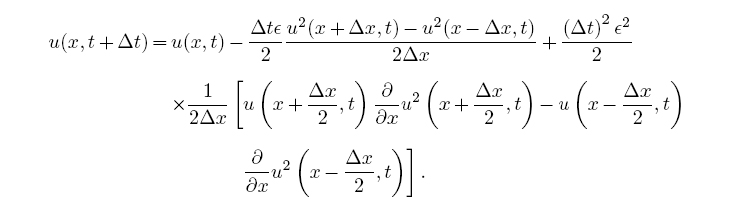
We next substitute these derivatives into the Taylor expansion (19.10) to obtain

We now replace the outer x derivatives by central differences of spacing Δ x/2:

Next we approximate u(x ± Δ x/2,t) by the average of adjacent grid points,

and apply a central-difference approximation to the second derivatives:

Finally, putting all these derivatives together yields the discrete form

where we have substituted the CFL number β. This Lax–Wendroff scheme is explicit, centered upon the grid points, and stable for β < 1 (small nonlinearities).

19.3.2 Implementation and Assessment of Burgers’ Shock Equation

The listing below presents the essentials of the Lax–Wendroff method.

19.4 Including Dispersion

We have just seen that Burgers’ equation can turn an initially smooth wave into a square-edged shock wave. An inverse wave phenomenon is dispersion, in which a waveform disperses or broadens as it travel through a medium. Dispersion does not cause waves to lose energy and attenuate but rather to lose information with time.Physically,dispersion may arise when the propagating medium has structures with a spatial regularity equal to some fraction of a wavelength. Mathematically, dispersion may arise from terms in the wave equation that contain higher-order space derivatives. For example, consider the waveform

corresponding to a plane wave traveling to the right (“traveling” because the phase kx -ωt remains unchanged if you increase x with time). When this u(x, t) is substituted into the advection equation (19.4), we obtain

This equation is an example of a dispersion relation, that is, a relation between frequency ω and wave vector k. Because the group velocity of a wave

the linear dispersion relation (19.14) leads to all frequencies having the same group velocity c and thus dispersionless propagation.

Let us now imagine that a wave is propagating with a small amount of dispersion, that is, with a frequency that has some what less than a linear increase with the wave number k:

Note that we skip the even powers in (19.16), so that the group velocity,

is the same for waves traveling to the left the or the right. If plane-wave solutions like (19.13) were to arise from a wave equation, then (as verified by substitution) the ω term of the dispersion relation (19.16) would arise from a first-order time derivative, the ck term from a first-order space derivative, and the k³ term from a third-order space derivative:

We leave it as an exercise to show that solutions to this equation do indeed have waveforms that disperse in time.

19.5 Shallow-Water Solitons, the KdeV Equation

In this section we look at shallow-water soliton waves. Though including some complications, this subject is fascinating and is one for which the computer has been absolutely essential for discovery and understanding. In addition, we recommend that you look at some of the soliton animation we have placed in the animations folder on the CD (available online: http://press.princeton.edu/landau_survey/).

Figure 19.2 A single two-level waveform at time zero progressively breaks up into eight solitons (labeled) as time increases. The tallest soliton (1) is narrower and faster in its motion to the right.

We want to understand the unusual water waves that occur in shallow, narrow channels such as canals [Abar 93, Tab 89]. The analytic description of this “heap of water” was given by Korteweg and deVries (KdeV) [KdeV 95] with the partial differential equation

As we discussed in §19.1 in our study of Burgers’ equation, the nonlinear term εu ∂u/∂t leads to a sharpening of the wave and ultimately a shock wave. In contrast, as we discussed in our study of dispersion, the ∂3u/∂x³ term produces broadening. These together with the ∂u/∂t term produce traveling waves. For the proper parameters and initial conditions, the dispersive broadening exactly balances the nonlinear narrowing, and a stable traveling wave is formed.

KdeV solved (19.19) analytically and proved that the speed (19.1) given by Russell is in fact correct. Seventy years after its discovery, the KdeV equation was rediscovered by Zabusky and Kruskal [Z&K 65], who solved it numerically and found that a cos(x/L) initial condition broke up into eight solitary waves (Figure 19.2). They also found that the parts of the wave with larger amplitudes moved faster than those with smaller amplitudes, which is why the higher peaks tend to be on the right in Figure 19.2. As if wonders never cease, Zabusky and Kruskal, who coined the name soliton for the solitary wave, also observed that a faster peak actually passed through a slower one unscathed (Figure 19.3).

Figure 19.3 Two shallow-water solitary waves crossing each other (computed with the code SolCross.java on the instructor’s CD: http://press.princeton.edu/landau_survey/). The taller soliton on the left catches up with and overtakes the shorter one at ≃ 5.

19.5.1 Analytic Soliton Solution

The trick in analytic approaches to these types of nonlinear equations is to substitute a guessed solution that has the form of a traveling wave,

This form means that if we move with a constant speed c, we will see a constant wave form (but now the speed will depend on the magnitude of u). There is no guarantee that this form of a solution exists, but it is a lucky guess because substitution into the KdeV equation produces a solvable ODE and its solution:

where ξ₀ is the initial phase. We see in (19.22) an amplitude that is proportional to the wave speed c, and a sech² function that gives a single lumplike wave. This is a typical analytic form for a soliton.

19.5.2 Algorithm for KdeV Solitons

The KdeV equation is solved numerically using a finite-difference scheme with the time and space derivatives given by central-difference approximations:

To approximate ∂³u(x,t)/∂x³, we expand u(x,t) to O(Δt)³ about the four points u(x ± 2Δ x, t) and u(x ± Δx, t),

which we solve for ∂3u(x,t)/∂x3. Finally, the factor u(x,t) in the second term of (19.19) is taken as the average of three x values all with the same t:

These substitutions yield the algorithm for the KdeV equation:

To apply this algorithm to predict future times, we need to know u(x, t) at present and past times. The initial-time solution ui,₁ is known for all positions i via the initial condition. To find ui,₂, we use a forward-difference scheme in which we expand u(x, t), keeping only two terms for the time derivative:

The keen observer will note that there are still some undefined columns of points, namely, u_1,j, u_2,j, u_Nmax-1,j, and u_{N max} ,_j, where N_max is the total number of grid points. A simple technique for determining their values is to assume that u₁,₂ = 1 and u_{N max},2 = 0. To obtain u2,2 and u_Nmax-1,₂, assume that u_i+_2,2 = u_i+_1,2 and u_i-2,2 = u_i-1,2 (avoid u_i+2,2 for i = N _max - 1, and ui-2,2 for i = 2). To carry out these steps, approximate (19.27) so that

The truncation error and stability condition for our algorithm are related:

The first equation shows that smaller time and space steps lead to a smaller approximation error, yet because round-off error increases with the number of steps, the total error does not necessarily decrease (Chapter 2, “Errors & Uncertainties in Computations). Yet we are also limited in how small the steps can be made by the stability condition (19.29), which indicates that making Δx too small always leads to instability. Care and experimentation are required.

19.5.3 Implementation: KdeV Solitons

Modify or run the program Soliton.java in Listing 19.2 that solves the KdeV equation (19.19) for the initial condition

with parameters e = 0.2 and µ = 0.1. Start with Δx = 0.4 and Δt = 0.1. These constants are chosen to satisfy (19.28) with |u| = 1.

Listing 19.2 Soliton.java solves the KdeV equation for 1-D solitons corresponding to a “bore” initial conditions.

19.5.4 Exploration: Solitons in Phase Space and Crossing

19.6 Unit II. River Hydrodynamics

Problem: In order to give migrating salmon a place to rest during their arduous upstream journey, the Oregon Department of Environment is thinking of placing objects in several deep, wide, fast-flowing streams. One such object is a long beam of rectangular cross section (Figure 19.4 left), and another is a set of plates (Figure 19.4 right). The objects are far enough below the surface so as not to disturb the surface flow, and far enough from the bottom of the stream so as not to disturb the flow there either.

Your problem is to determine the spatial dependence of the stream’s velocity and, specifically, whether the wake of the object will be large enough to provide a resting place for a meter-long salmon.

19.7 Hydrodynamics, the Navier–Stokes Equation (Theory)

We continue with the assumption made in Unit I that water is incompressible and thus that its density ρ is constant. We also simplify the theory by looking only at steady-state situations, that is, ones in which the velocity is not a function of time. However, to understand how water flows around objects, like our beam, it is essential to include the complication of frictional forces (viscosity).

For the sake of completeness, we repeat here the first equation of hydrodynamics, the continuity equation (19.2):

Before proceeding to the second equation, we introduce a special time derivative, the hydrodynamic derivative Dv/Dt, which is appropriate for a quantity contained in a moving fluid [F&W 80]:

Figure 19.4 Cross-sectional view of the flow of a stream around a submerged beam (left) and two parallel plates (right). Both beam and plates have length L along the direction of flow. The flow is seen to be symmetric about the centerline and to be unaffected at the bottom and surface by the submerged object.

This derivative gives the rate of change, as viewed from a stationary frame, of the velocity of material in an element of fluid and so incorporates changes due to the motion of the fluid (first term) as well as any explicit time dependence of the velocity. Of particular interest is that Dv/Dt is second order in the velocity, and so its occurrence reflects nonlinearities into the theory. You may think of these nonlinearities as related to the fictitious (inertial) forces that would occur if we tried to describe the motion in the fluid’s rest frame (an accelerating frame).

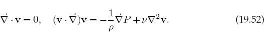
The material derivative is the leading term in the Navier–Stokes equation,

Here ν is the kinematic viscosity, P is the pressure, and (19.33) shows the derivatives in Cartesian coordinates. This equation describes transfer of the momentum of the fluid within some region of space as a result of forces and flow (think dp/dt = F), there being a simultaneous equation for each of the three velocity components. The v .∇v term in Dv/Dt describes transport of momentum in some region of space resulting from the fluid’s flow and is often called the convection or advection term.² The P term describes the velocity change as a result of pressure changes, and the ν∇²v term describes the velocity change resulting from viscous forces (which tend to dampen the flow).

The explicit functional dependence of the pressure on the fluid’s density and temperature P(ρ, T, x) is known as the equation of state of the fluid and would have to be known before trying to solve the Navier–Stokes equation. To keep our problem simple we assume that the pressure is independent of density and temperature, which leaves the four simultaneous partial differential equations (19.30) and (19.32) to solve. Because we are interested in steady-state flow around an object, we assume that all time derivatives of the velocity vanish. Because we assume that the fluid is incompressible, the time derivative of the density also vanishes, and (19.30) and (19.32) become

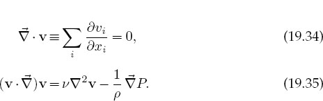
The first equation expresses the equality of inflow and outflow and is known as the condition of incompressibility. In as much as the stream in our problem is much wider than the width (z dimension) of the beam and because we are staying away from the banks, we will ignore the z dependence of the velocity. The explicit PDEs we need to solve are then:

Figure 19.5 The boundary conditions for two thin submerged plates. The surrounding box is the integration volume within which we solve the PDEs and upon whose surface we impose the boundary conditions. In practice the box is much larger than L and H.

19.7.1 Boundary Conditions for Parallel Plates

The plate problem is relatively easy to solve analytically, and so we will do it! This will give us some experience with the equations as well as a check for our numerical solution. To find a unique solution to the PDEs (19.36)–(19.38), we need to specify boundary conditions. As far as we can tell, picking boundary conditions is some what of an acquired skill, and it becomes easier with experience (similar to what happens after solving hundreds of electrostatics problems). Some of the boundary conditions apply to the flow at the surfaces of submerged objects, while others apply to the “box” or tank that surrounds the fluid. As we shall see, sometimes these boundary conditions relate to the velocities directly, while at other times they relate to the derivatives of the velocities.

We assume that the submerged parallel plates are placed in a stream that is flowing with a constant velocity V₀ in the horizontal direction (Figure 19.4 right). If the velocity V₀ is not too high or the kinematic viscosity ν is sufficiently large, then the flow should be smooth and without turbulence. We call such flow laminar. Typically, a fluid undergoing laminar flow moves in smooth paths that do not close on themselves, like the smooth flow of water from a faucet. If we imagine attaching a vector to each element of the fluid, then the path swept out by that vector is called a streamline or line of motion of the fluid. These streamlines can be visualized experimentally by adding a colored dye to the stream. We assume that the plates are so thin that the flow remains laminar as it passes around and through them.

If the plates are thin, then the flow upstream of them is not affected, and we can limit our solution space to the rectangular region in Figure 19.5. We assume that the length L and separation H of the plates are small compared to the size of the stream, so the flow returns to uniform as we get far downstream from the plates. As seen in Figure 19.5, there are boundary conditions at the inlet where the fluid enters our solution space, at the outlet where it leaves, and at the stationary plates. In addition, since the plates are far from the stream’s bottom and surface, we may assume that the dotted-dashed centerline is a plane of symmetry, with identical flow above and below the plane. We thus have four different types of boundary conditions to impose on our solution:

Solid plates: Since there is friction (viscosity) between the fluid and the plate surface, the only way to have laminar flow is to have the fluid’s velocity equal to the plate’s velocity, which means both are zero:

Such being the case, we have smooth flow in which the negligibly thin plates lie along streamlines of the fluid (like a “streamlined” vehicle).

Inlet: The fluid enters the integration domain at the in let with a horizontal velocity V₀. Since the inlet is far upstream from the plates, we assume that the fluid velocity at the inlet is unchanged:

Outlet: Fluid leaves the integration domain at the outlet. While it is totally reasonable to assume that the fluid returns to its unperturbed state there, we are not told what that is. So, instead, we assume that there is a physical outlet at the end with the water just shooting out of it. Consequently, we assume that the water pressure equals zero at the outlet (as at the end of a garden hose) and that the velocity does not change in a direction normal to the outlet:

Symmetry plane: If the flow is symmetric about the y = 0 plane, then there cannot be flow through the plane and the spatial derivatives of the velocity components normal to the plane must vanish:

This condition follows from the assumption that the plates are along streamlines and that they are negligibly thin. It means that all the streamlines are parallel to the plates as well as to the water surface, and so it must be that vy = 0 everywhere. The fluid enters in the horizontal direction, the plates do not change the vertical y component of the velocity, and the flow remains symmetric about the centerline. There is a retardation of the flow around the plates due to the viscous nature of the flow and due to the v = 0 boundary layers formed on the plates, but there are no actual vy components.

19.7.2 Analytic Solution for Parallel Plates

For steady flow around and through the parallel plates, with the boundary conditions imposed and v_y = 0, the continuity equation (19.36) reduces to

This tells us that vx does not vary with x. With these conditions, the Navier–Stokes equations (19.38) in x and y reduce to the linear PDEs

(Observe that if the effect of gravity were also included in the problem, then the pressure would increase with the depth y.) Since the LHS of the first equation describes the x variation, and the RHS the y variation, the only way for the equation to be satisfied in general is if both sides are constant:

Double integration of the second equation with respect to y and replacement of the constant by ∂P/∂x yields

where C₁ and C₂ are constants. The values of C₁ and C₂ are determined by requiring the fluid to stop at the plate, v_x(0) = v_x(H) = 0, where H is the distance between plates. This yields

Because ∂P/∂y = 0, the pressure does not vary with y. The continuity and smoothness of P over the region,

are a consequence of laminar flow. Such being the case, we may assume that ∂P/∂x has no y dependence, and so (19.42) describes a velocity profile varying as y2.

A check on our numerical CFD simulation ensures that it also gives a parabolic velocity profile for two parallel plates. To be even more precise, we can determine ∂P/∂x for this problem and thereby produce a purely numerical answer for comparison. To do that we examine a volume of current that at the inlet starts out with 0 ≤y ≤ H. Because there is no vertical component to the flow, this volume ends up flowing between the plates. If the volume has a unit z width, then the mass flow (mass/unit time) at the inlet is

When the fluid is between the plates, the velocity has a parabolic variation in height y. Consequently, we integrate over the area of the plates without changing the net mass flow between the plates:

Yet we know that Q = ρHVo, and substitution gives us an expression for how the pressure gradient depends upon the plate separation:

We see that there is a pressure drop as the fluid flows through the plates and that the drop increases as the plates are brought closer together (the Bernoulli effect). To program the equations, we assign the values VQ = 1 m/s (2.24mi/h), ρ=1 kg/m (≥air), ν = 1 m²/s (somewhat less viscous than glycerin), and H=1m (typical boulder size):

19.7.3 Finite-Difference Algorithm and Overrelaxation

Now we develop an algorithm for solution of the Navier–Stokes and continuity PDEs using successive overrelaxation. This is a variation of the method used in Chapter 17, “PDEs for Electrostatics & Heat Flow,” to solve Poisson’s equation. We divide space into a rectangular grid with the spacing h in both the x and y directions:

We next express the derivatives in (19.36)–(19.38) as finite differences of the values of the velocities at the grid points using central-difference approximations.

For ν = 1 m²/s and ρ = 1kg/m³, this yields

Since v^y ≡ 0 for this problem, we rearrange terms to obtain for v^x:

We recognize in(19.48) an algorithm similar to the one we used in solving Laplace’s equation by relaxation. Indeed, as we did there, we can accelerate the convergence by writing the algorithm with the new value of vx given as the old value plus a correction (residual):

As done with the Poisson equation algorithm, successive iterations sweep the interior of the grid, continuously adding in the residual (19.49) until the change becomes smaller than some set level of tolerance, |r_i,j| < ε.

A variation of this method, successive overrelaxation, increases the speed at which the residuals approach zero via an amplifying factor ω:

The standard relaxation algorithm (19.49) is obtained with ω = 1, an accelerated convergence (overrelaxation) is obtained with ω ≥ 1, and underrelaxation occurs for ω < 1. Values ω > 2 lead to numerical instabilities and so are not recommended. Although a detailed analysis of the algorithm is necessary to predict the optimal value for ω, we suggest that you test different valuesfor ω to see which one provides the fastest convergence for your problem.

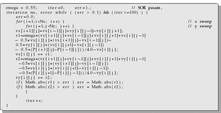
19.7.4 Successive Overrelaxation Implementation

Here is a program fragment that implements SOR for v^x and v^y:

19.8 2-D Flow over a Beam

Now that the comparison with an analytic solution has shown that our CFD simulation works, we return to determining if the beam in Figure 19.4 might produce a good resting place for salmon. While we have no analytic solution with which to compare, our canoeing and fishing adventures have taught us that standing waves with fish in them are often formed behind rocks in streams, and so we expect there will be a standing wave formed behind the beam.

19.9 Theory: Vorticity Form of the Navier–Stokes Equation

We have seen how to solve numerically the hydrodynamics equations

These equations determine the components of a fluid’s velocity, pressure, and density as functions of position. In analogy to electrostatics, where one usually solves for the simpler scalar potential and then takes its gradient to determine the more complicated vector field, we now recast the hydrodynamic equations into forms that permit us to solve two simpler equations for simpler functions, from which the velocity is obtained via a gradient operation.³

We introduce the stream function u(x) from which the velocity is determined by the curl operator:

Note the absence of the z component of velocity v for our problem. Since . ( × u) ≡ 0, we see that any v that can be written as the curl of u automatically satisfies the continuity equation . v = 0. Further, since v for our problem has only x and y components, u(x) needs to have only a z component:

(Even though the vorticity has just one component, it is a pseudoscalar and not a scalar because it reverses sign upon reflection.) It is worth noting that in 2-D flows, the contour lines u = constant are the streamlines.

The second simplifying function is the vorticity field w(x), which is related physically and alphabetically to the angular velocity ω of the fluid. Vorticity is defined as the curl of the velocity (sometimes with a — sign):

Because the velocity in our problem does not change in the z direction, we have

Physically, we see that the vorticity is a measure of how much the fluid’s velocity curls or rotates, with the direction of the vorticity determined by the right-hand rule for rotations. In fact, if we could pluck a small element of the fluid into space (so it would not feel the internal strain of the fluid), we would find that it is rotating like a solid with angular velocity w ∝ w [Lamb 93]. That being the case, it is useful to think of the vorticity as giving the local value of the fluid’s angular velocity vector. If w = 0, we have irrotational flow.

The field lines of w are continuous and move as if attached to the particles of the fluid. A uniformly flowing fluid has vanishing curl, while a nonzero vorticity indicates that the current curls back on itself or rotates. From the definition of the stream function (19.53), we see that the vorticity w is related to it by

where we have used a vector identity for × ( × u). Yet the divergence .u = 0 since u has only a z component that does not vary with z (or because there is no source for u). We have now obtained the basic relation between the stream function u and the vorticity w:

Equation (19.58) is analogous to Poisson’s equation of electrostatics, Δ²ø= −4πρ, only now each component of vorticity w is a source for the corresponding component of the stream function u. If the flow is irrotational, that is, if w = 0, then we need only solve Laplace’s equation for each component of u. Rotational flow, with its coupled nonlinearities equations, leads to more interesting behavior.

As is to be expected from the definition of w, the vorticity form of the Navier–Stokes equation is obtained by taking the curl of the velocity form, that is, by operating on both sides with ×. After significant manipulations we obtain

This and (19.58) are the two simultaneous PDEs that we need to solve. In 2-D, with u and w having only z components, they are

So after all that work, we end up with two simultaneous, nonlinear, elliptic PDEs for the functions w(x, y) and u(x, y) that look like a mixture of Poisson’s equation with the frictional and variable-density terms of the wave equation. The equation for u is Poisson’s equation with source w and must be solved simultaneously with the second.It is this second equation that contains mixed products of the derivatives of u and w and thus introduces nonlinearity.

19.9.1 Finite Differences and the SOR Algorithm

We solve (19.60) and (19.61) on an N_x ×N_y grid of uniform spacing h with

Since the beam is symmetric about its centerline (Figure 19.4 left), we need the solution only in the upper half-plane. We apply the now familiar central-difference approximation to the Laplacians of u and w to obtain the difference equation

Likewise, for the first derivatives,

The difference form of the vorticity Navier–Stokes equation (19.60) becomes

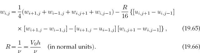
Note that we have placed u_i,j and w_i,j on the LHS of the equations in order to obtain an algorithm appropriate to solution by relaxation.

The parameter R in (19.66) is related to the Reynolds number. When we solve the problem in natural units, we measure distances in units of grid spacing h, velocities in units of initial velocity V₀, stream functions in units of V₀h, and vorticity in units of V₀/h. The second form is in regular units and is dimensionless. This R is known as the grid Reynolds number and differs from the physical R, which has a pipe diameter in place of the grid spacing h.

The grid Reynolds number is a measure of the strength of the coupling of the nonlinear terms in the equation. When R is small, the viscosity acts as a frictional force that damps out fluctuations and keeps the flow smooth. When the physical R is large (R ~ 2000), physical fluids undergo phase transitions from laminar to turbulent flow in which turbulence occurs at a cascading set of smaller and smaller space scales [Rey 83]. However, simulations that produce the onset of turbulence have been a research problem since Reynolds first experiments in 1883 [Rey 83, F&S], possibly because laminar flow simulations are stable against small perturbations and some large-scale “kick” appears necessary to change laminar to turbulent flow. Recent research along these lines have been able to find unstable, traveling-wave solutions to the Navier–Stokes equations, and the hope is that these may lead to a turbulent transition [Fitz 04].

As discussed in §19.7.3, the finite-difference algorithm can have its convergence accelerated by the use of successive overrelaxation (19.64):

Here ω is the overrelaxation parameter and should lie in the range 0 < ω < 2 for stability. The residuals are just the changes in a single step, r⁽¹⁾ = u^new - u^old and r(2) =w^new -w^old:

Figure 19.6 Boundary conditions for flow around the beam in Figure 19.4. The flow is symmetric about the centerline, and the beam has length L in the x direction (along flow).

19.9.2 Boundary Conditions for a Beam

A well-defined solution of these elliptic PDEs requires a combination of (less than obvious) boundary conditions on u and w. Consider Figure 19.6, based on the analysis of [Koon 86]. We assume that the inlet, outlet, and surface are far from the beam, which may not be evident from the not-to-scale figure.

Freeflow: If there were no beam in the stream, then we would have free flow with the entire fluid possessing the inlet velocity:

(Recollect that we can think of w = 0 as indicating no fluid rotation.) The centerline divides the system along a symmetry plane with identical flow above and below it. If the velocity is symmetric about the centerline, then its y component must vanish there:

Centerline: The centerline is a streamline with u = constant because there is no velocity component perpendicular to it. We set u = 0 according to (19.69). Because there cannot be any fluid flowing into or out of the beam, the normal component of velocity must vanish along the beam surfaces. Consequently, the streamline u = 0 is the entire lower part of Figure 19.6, that is, the centerline and the beam surfaces. Likewise, the symmetry of the problem permits us to set the vorticity w = 0 along the centerline.

Inlet: At the inlet, the fluid flow is horizontal with uniform x component V₀ at all heights and with no rotation:

Surface: We are told that the beam is sufficiently submerged so as not to disturb the flow on the surface of the stream. Accordingly, we have free-flow conditions on the surface:

Outlet: Unless something truly drastic is happening, the conditions on the far downstream outlet have little effect on the far upstream flow. A convenient choice is to require the stream function and vorticity to be constant:

Beamsides: We have already noted that the normal component of velocity v^x and stream function u vanish along the beam surfaces. In addition, becausethe flow is viscous, it is also true that the fluid “sticks” to the beam somewhat and so the tangential velocity also vanishes along the beam’s surfaces. While these may all be true conclusions regarding the flow, specifying them as boundary conditions would overrestrict the solution (see Table 17.1 for elliptic equations) to the point where no solution may exist. Accordingly, we simply impose the no-slip boundary condition on the vorticity w. Consider a grid point (x, y) on the upper surface of the beam. The stream function u at a point (x, y +h) above it can be related via a Taylor series in y:

Because w has only a z component, it has a simple relation to ∇×v:

Because of the fluid’s viscosity, the velocity is stationary along the beam top:

Because the current flows smoothly along the top of the beam, v^y must also vanish. In addition, since there is no x variation, we have

After substituting these relations into the Taylor series (19.74), we can solve for w and obtain the finite-difference version of the top boundary condition:

  Similar treatments applied to other surfaces yield the following boundary conditions.

19.9.3 SOR on a Grid Implementation

Beam.java in Listing 19.3 is our solution of the vorticity form of the Navier–Stokes equation. You will notice that while the relaxation algorithm is rather simple, some care is needed in implementing the many boundary conditions. Relaxation of the stream function andof the vorticity is done by separate methods, and the file output format is that for a Gnuplot surface plot.

Listing 19.3 Beam.java solves the Navier–Stokes equation for the flow over a plate.

Figure 19.7 Left: Gnuplot surface plot with contours of the stream function u for R = 5. Right: Contours of stream function for R= 1 visualized with colors by OpenDX.

19.9.4 Assessment

19.9.5 Exploration

1 We acknowledge some helpful reading of Unit I by Satoru S. Kano.

2 We discuss pure advection in §19.1. In oceanology or meteorology, convection implies the transfer of mass in the vertical direction where it overcomes gravity, whereas advection refers to transfer in the horizontal direction.

3 If we had to solve only the simpler problem of irrotational flow (no turbulence), then we wouldbe abletouseascalar velocity potential,inclose analogytoelectrostatics [Lamb 93]. For the more general rotational flow, two vector potentials are required.