9 Channel Equalization

Search in book...
Toggle Font Controls
Create new playlist

Name your new playlist

Playlist description (optional)
Sign In

Email address

Password

Forgot Password?

or

Continue with Facebook

Continue with Google
Sign Up

Full Name

Email address

Confirm Email Address

Password

or

Continue with Facebook

Continue with Google

9 Channel Equalization

John G. Proakis

9.1 Characterization of Channel Distortion

9.2 Characterization of Intersymbol Interference

9.3 Linear Equalizers

Adaptive Linear Equalizers

9.4 Decision-Feedback Equalizer

9.5 Maximum-Likelihood Sequence Detection

9.6 Conclusions

References

9.1 Characterization of Channel Distortion

Many communication channels, including telephone channels and some radio channels, may be generally characterized as band-limited linear filters. Consequently, such channels are described by their frequency response C(f), which may be expressed as

C (f) = A (f) e^{j θ (f)} (9.1)

$C (f) = A (f) e^{j θ (f)} (9.1)$

where A( f ) is called the amplitude response and θ( f ) is called the phase response. Another characteristic that is sometimes used in place of the phase response is the envelope delay or group delay, which is defined as

τ (f) = - \frac{1}{2 π} \frac{d θ (f)}{d f} (9.2)

$τ (f) = - \frac{1}{2 π} \frac{d θ (f)}{d f} (9.2)$

A channel is said to be nondistorting or ideal if, within the bandwidth W occupied by the transmitted signal, A( f ) = const and θ( f ) is a linear function of frequency [or the envelope delay τ( f ) = const]. On the other hand, if A( f ) and τ( f ) are not constant within the bandwidth occupied by the transmitted signal, the channel distorts the signal. If A( f ) is not constant, the distortion is called amplitude distortion and if τ( f ) is not constant, the distortion on the transmitted signal is called delay distortion.

As a result of the amplitude and delay distortion caused by the nonideal channel frequency response characteristic C( f ), a succession of pulses transmitted through the channel at rates comparable to the bandwidth W are smeared to the point that they are no longer distinguishable as well-defined pulses at the receiving terminal. Instead, they overlap and, thus, we have intersymbol interference (ISI). As an example of the effect of delay distortion on a transmitted pulse, Figure 9.1a illustrates a band-limited pulse having zeros periodically spaced in time at points labeled ±T, ±2T, and so on. If information is conveyed by the pulse amplitude, as in pulse amplitude modulation (PAM), for example, then one can transmit a sequence of pulses, each of which has a peak at the periodic zeros of the other pulses. Transmission of the pulse through a channel modeled as having a linear envelope delay characteristic τ( f ) [quadratic phase θ( f )], however, results in the received pulse shown in Figure 9.1b having zero crossings that are no longer periodically spaced. Consequently, a sequence of successive pulses would be smeared into one another, and the peaks of the pulses would no longer be distinguishable. Thus, the channel delay distortion results in intersymbol interference. As is discussed in this chapter, it is possible to compensate for the nonideal frequency response characteristic of the channel by use of a filter or equalizer at the demodulator. Figure 9.1c illustrates the output of a linear equalizer that compensates for the linear distortion in the channel.

Images

FIGURE 9.1 Effect of channel distortion: (a) channel input, (b) channel output, and (c) equalizer output.

The extent of the intersymbol interference on a telephone channel can be appreciated by observing a frequency response characteristic of the channel. Figure 9.2 illustrates the measured average amplitude and delay as a function of frequency for a medium-range (180–725 mi) telephone channel of the switched telecommunications network as given by Duffy and Tratcher, 1971. We observe that the usable band of the channel extends from about 300 to about 3000 Hz. The corresponding impulse response of the average channel is shown in Figure 9.3. Its duration is about 10 ms. In comparison, the transmitted symbol rates on such a channel may be of the order of 2500 pulses or symbols per second. Hence, intersymbol interference might extend over 20–30 symbols.

Besides telephone channels, there are other physical channels that exhibit some form of time dispersion and, thus, introduce intersymbol interference. Radio channels, such as short-wave ionospheric propagation (HF), tropospheric scatter, and mobile cellular radio are three examples of time-dispersive wireless channels. In these channels, time dispersion and, hence, intersymbol interference is the result of multiple propagation paths with different path delays. The number of paths and the relative time delays among the paths vary with time and, for this reason, these radio channels are usually called time-variant multipath channels. The time-variant multipath conditions give rise to a wide variety of frequency response characteristics. Consequently, the frequency response characterization that is used for telephone channels is inappropriate for time-variant multipath channels. Instead, these radio channels are characterized statistically in terms of the scattering function, which, in brief, is a two-dimensional representation of the average received signal power as a function of relative time delay and Doppler frequency (see Proakis [4]).

Images

FIGURE 9.2 Average amplitude and delay characteristics of medium-range telephone channel.

Images

FIGURE 9.3 Impulse response of average channel with amplitude and delay shown in Figure 9.2.

For illustrative purposes, a scattering function measured on a medium-range (150 mi) tropospheric scatter channel is shown in Figure 9.4. The total time duration (multipath spread) of the channel response is approximately 0.7 µs on the average, and the spread between half-power points in Doppler frequency is a little less than 1 Hz on the strongest path and somewhat larger on the other paths. Typically, if one is transmitting at a rate of 10⁷ symbols/s over such a channel, the multipath spread of 0.7 µs will result in intersymbol interference that spans about seven symbols.

Images

FIGURE 9.4 Scattering function of a medium-range tropospheric scatter channel.

9.2 Characterization of Intersymbol Interference

In a digital communication system, channel distortion causes intersymbol interference, as illustrated in the preceding section. In this section, we shall present a model that characterizes the ISI. The digital modulation methods to which this treatment applies are PAM, phase-shift keying (PSK), and quadrature amplitude modulation (QAM). The transmitted signal for these three types of modulation may be expressed as

\begin{matrix} s (t) = υ_{c} (t) \cos 2 π f_{c} t - υ_{s} (t) \sin 2 π f_{c} t \\ = Re [υ (t) e^{j 2 π f_{c} t}] \end{matrix} (9.3)

$\begin{matrix} s (t) = υ_{c} (t) \cos 2 π f_{c} t - υ_{s} (t) \sin 2 π f_{c} t \\ = Re [υ (t) e^{j 2 π f_{c} t}] \end{matrix} (9.3)$

where υ(t) = υ_c(t) + jυ_s(t) is called the equivalent low-pass signal, f_c is the carrier frequency, and Re[ ] denotes the real part of the quantity in brackets.

In general, the equivalent low-pass signal is expressed as

υ (t) = \sum_{n = 0}^{\infty} I_{n} g_{T} (t - n T) (9.4)

$υ (t) = \sum_{n = 0}^{\infty} I_{n} g_{T} (t - n T) (9.4)$

where g_T(t) is the basic pulse shape that is selected to control the spectral characteristics of the transmitted signal, {I_n} the sequence of transmitted information symbols selected from a signal constellation consisting of M points, and T the signal interval (1/T is the symbol rate). For PAM, PSK, and QAM, the values of I_n are points from M-ary signal constellations. Figure 9.5 illustrates the signal constellations for the case of M = 8 signal points. Note that for PAM, the signal constellation is one dimensional. Hence, the equivalent low-pass signal υ(t) is real valued, that is, υ_s(t) = 0 and υ_c(t) = υ(t). For M-ary (M > 2) PSK and QAM, the signal constellations are two dimensional and, hence, υ(t) is complex valued.

The signal s(t) is transmitted over a bandpass channel that may be characterized by an equivalent low-pass frequency response C(f). Consequently, the equivalent low-pass received signal can be represented as

r (t) = \sum_{n = 0}^{\infty} I_{n} h (t - n T) + w (t) (9.5)

$r (t) = \sum_{n = 0}^{\infty} I_{n} h (t - n T) + w (t) (9.5)$

where h(t) = g_T(t)*c(t), and c(t) is the impulse response of the equivalent low-pass channel, the asterisk denotes convolution, and w(t) represents the additive noise in the channel.

To characterize the ISI, suppose that the received signal is passed through a receiving filter and then sampled at the rate of 1/T samples/s. In general, the optimum filter at the receiver is matched to the received signal pulse h(t). Hence, the frequency response of this filter is H*(f). We denote its output as

y (t) = \sum_{n = 0}^{\infty} I_{n} x (t - n T) + ν (t) (9.6)

$y (t) = \sum_{n = 0}^{\infty} I_{n} x (t - n T) + ν (t) (9.6)$

Images

FIGURE 9.5 M = 8 signal constellations for (a) PAM, (b) PSK, and (c) QAM.

where x(t) is the signal pulse response of the receiving filter, that is, X(f) = H(f)H*(f) = |H(f)|², and ν(t) is the response of the receiving filter to the noise w(t). Now, if y(t) is sampled at times t = kT, k = 0, 1, 2, …, we have

\begin{matrix} y (k T) \equiv y_{k} = \sum_{n = 0}^{\infty} I_{n} x (k T - n T) + ν (k T) \\ = \sum_{n = 0}^{\infty} I_{n} x_{k - n} + ν_{k}, k = 0, 1, \dots \end{matrix} (9.7)

$\begin{matrix} y (k T) \equiv y_{k} = \sum_{n = 0}^{\infty} I_{n} x (k T - n T) + ν (k T) \\ = \sum_{n = 0}^{\infty} I_{n} x_{k - n} + ν_{k}, k = 0, 1, \dots \end{matrix} (9.7)$

The sample values {y_k} can be expressed as

y_{k} = x_{0} (I_{k} + \frac{1}{x_{0}} \sum_{\begin{array}{l} n = 0 \\ n \neq k \end{array}}^{\infty} I_{n} x_{k - n}) + ν_{k}, k = 0, 1, \dots (9.8)

$y_{k} = x_{0} (I_{k} + \frac{1}{x_{0}} \sum_{\begin{array}{l} n = 0 \\ n \neq k \end{array}}^{\infty} I_{n} x_{k - n}) + ν_{k}, k = 0, 1, \dots (9.8)$

The term x₀ is an arbitrary scale factor, which we arbitrarily set equal to unity for convenience. Then

y_{k} = I_{k} + \sum_{\begin{array}{l} n = 0 \\ n \neq k \end{array}}^{\infty} I_{n} x_{k - n} + ν_{k} (9.9)

$y_{k} = I_{k} + \sum_{\begin{array}{l} n = 0 \\ n \neq k \end{array}}^{\infty} I_{n} x_{k - n} + ν_{k} (9.9)$

The term I_k represents the desired information symbol at the kth sampling instant, the term

\sum_{\begin{array}{l} n = 0 \\ n \neq k \end{array}}^{\infty} I_{n} x_{k - n} (9.10)

$\sum_{\begin{array}{l} n = 0 \\ n \neq k \end{array}}^{\infty} I_{n} x_{k - n} (9.10)$

represents the ISI, and ν_k is the additive noise variable at the kth sampling instant.

The amount of ISI, and noise in a digital communication system can be viewed on an oscilloscope. For PAM signals, we can display the received signal y(t) on the vertical input with the horizontal sweep rate set at 1/T. The resulting oscilloscope display is called an eye pattern because of its resemblance to the human eye. For example, Figure 9.6 illustrates the eye patterns for binary and four-level PAM modulation. The effect of ISI is to cause the eye to close, thereby reducing the margin for additive noise to cause errors. Figure 9.7 graphically illustrates the effect of ISI in reducing the opening of a binary eye. Note that intersymbol interference distorts the position of the zero crossings and causes a reduction in the eye opening. Thus, it causes the system to be more sensitive to a synchronization error.

For PSK and QAM, it is customary to display the eye pattern as a two-dimensional scatter diagram illustrating the sampled values {y_k} that represent the decision variables at the sampling instants. Figure 9.8 illustrates such an eye pattern for an 8-PSK signal. In the absence of intersymbol interference and noise, the superimposed signals at the sampling instants would result in eight distinct points corresponding to the eight transmitted signal phases. Intersymbol interference and noise result in a deviation of the received samples {y_k} from the desired 8-PSK signal. The larger the intersymbol interference and noise, the larger the scattering of the received signal samples relative to the transmitted signal points.

Images

FIGURE 9.6 Examples of eye patterns for binary and quaternary amplitude shift keying (or PAM).

Images

FIGURE 9.7 Effect of intersymbol interference on eye opening.

Images

FIGURE 9.8 Two-dimensional digital eye patterns. (a) Transmitted eight-phase signal and (b) received signal samples at the output of demodulation.

In practice, the transmitter and receiver filters are designed for zero ISI at the desired sampling times t = kT. Thus, if G_T(f) is the frequency response of the transmitter filter and G_R(f) is the frequency response of the receiver filter, then the product G_T(f) G_R(f) is designed to yield zero ISI.

For example, the product G_T(f) G_R(f) may be selected as

G_{T} (f) G_{R} (f) = X_{r c} (f) (9.11)

$G_{T} (f) G_{R} (f) = X_{r c} (f) (9.11)$

where X_rc(f) is the raised-cosine frequency response characteristic, defined as

X_{r c} (f) = {\begin{matrix} \begin{array}{l} T, \\ \frac{T}{2} 1 + \cos \frac{π T}{α} (| f | - \frac{1 - α}{2 T}), \\ 0, \end{array} & \begin{array}{l} 0 \leq | f | \leq \frac{(1 - α)}{2 T} \\ \frac{1 - α}{2 T} \leq | f | \leq \frac{1 + α}{2 T} \\ | f | > \frac{1 + α}{2 T} \end{array} \end{matrix} (9.12)

$X_{r c} (f) = {\begin{matrix} \begin{array}{l} T, \\ \frac{T}{2} 1 + \cos \frac{π T}{α} (| f | - \frac{1 - α}{2 T}), \\ 0, \end{array} & \begin{array}{l} 0 \leq | f | \leq \frac{(1 - α)}{2 T} \\ \frac{1 - α}{2 T} \leq | f | \leq \frac{1 + α}{2 T} \\ | f | > \frac{1 + α}{2 T} \end{array} \end{matrix} (9.12)$

Images

FIGURE 9.9 Pulses having a raised cosine spectrum. (a) Time response, (b) frequency response.

where α is called the rolloff factor, which takes values in the range 0 ≤ α ≤ 1, and 1/T is the symbol rate. The time response and frequency response are illustrated in Figure 9.9 for α = 0, 1/2, and 1. Note that when α = 0, X_rc(f) reduces to an ideal brick wall physically nonrealizable frequency response with bandwidth occupancy 1/2T. The frequency 1/2T is called the Nyquist frequency. For α > 0, the bandwidth occupied by the desired signal X_rc(f) beyond the Nyquist frequency 1/2T is called the excess bandwidth, and is usually expressed as a percentage of the Nyquist frequency. For example, when α = 1/2, the excess bandwidth is 50% and when α = 1, the excess bandwidth is 100%. The signal pulse x_rc(t) having the raised-cosine spectrum is

x_{r c} (t) = \frac{\sin π t / T}{π t / T} \frac{\cos (π α t / T)}{1 - 4 α^{2} t^{2} / T^{2}} (9.13)

$x_{r c} (t) = \frac{\sin π t / T}{π t / T} \frac{\cos (π α t / T)}{1 - 4 α^{2} t^{2} / T^{2}} (9.13)$

Figure 9.9b illustrates x_rc(t) for α = 0, 1/2, and 1. Note that x_rc(t) = 1 at t = 0 and x_rc(t) = 0 at t = kT, k = ±1, ±2, …. Consequently, at the sampling instants t = kT, k ≠ 0, there is no ISI from adjacent symbols when there is no channel distortion. In the presence of channel distortion, however, the ISI given by Equation 9.10 is no longer zero, and a channel equalizer is needed to minimize its effect on system performance.

9.3 Linear Equalizers

The most common type of channel equalizer used in practice to reduce SI is a linear transversal filter with adjustable coefficients {c_i}, as shown in Figure 9.10.

On channels whose frequency response characteristics are unknown, but time invariant, we may measure the channel characteristics and adjust the parameters of the equalizer; once adjusted, the parameters remain fixed during the transmission of data. Such equalizers are called preset equalizers. On the other hand, adaptive equalizers update their parameters on a periodic basis during the transmission of data and, thus, they are capable of tracking a slowly time-varying channel response.

Images

FIGURE 9.10 Linear transversal filter.

First, let us consider the design characteristics for a linear equalizer from a frequency domain viewpoint. Figure 9.11 shows a block diagram of a system that employs a linear filter as a channel equalizer.

The demodulator consists of a receiver filter with frequency response G_R(f) in cascade with a channel equalizing filter that has a frequency response G_E(f). As indicated in the preceding section, the receiver filter response G_R(f) is matched to the transmitter response, that is, $G_{R} (f) = G_{T}^{*} (f)$ $G_{R} (f) = G_{T}^{*} (f)$ , and the product G_R(f)G_T(f) is usually designed so that there is zero ISI at the sampling instants as, for example, when G_R(t)G_T(f) = X_rc(f).

For the system shown in Figure 9.11, in which the channel frequency response is not ideal, the desired condition for zero ISI is

G_{T} (f) C (f) G_{R} (f) G_{E} (f) = X_{r c} (f) (9.14)

$G_{T} (f) C (f) G_{R} (f) G_{E} (f) = X_{r c} (f) (9.14)$

where X_rc( f ) is the desired raised-cosine spectral characteristic. Since G_T(f)G_R(f) = X_rc(f) by design, the frequency response of the equalizer that compensates for the channel distortion is

G_{E} (f) = \frac{1}{C (f)} = \frac{1}{| C (f) |} e^{- j θ_{c} (f)} (9.15)

$G_{E} (f) = \frac{1}{C (f)} = \frac{1}{| C (f) |} e^{- j θ_{c} (f)} (9.15)$

Images

FIGURE 9.11 Block diagram of a system with an equalizer.

Thus, the amplitude response of the equalizer is |G_E( f )| = 1/|C( f )| and its phase response is θ_E( f ) = –θ_c( f ). In this case, the equalizer is said to be the inverse channel filter to the channel response.

We note that the inverse channel filter completely eliminates ISI caused by the channel. Since it forces the ISI to be zero at the sampling instants t = kT, k = 0, 1, …, the equalizer is called a zero-forcing equalizer. Hence, the input to the detector is simply

z_{k} = I_{k} + η_{k}, k = 0, 1, \dots (9.16)

$z_{k} = I_{k} + η_{k}, k = 0, 1, \dots (9.16)$

where η_k represents the additive noise and I_k is the desired symbol.

In practice, the ISI caused by channel distortion is usually limited to a finite number of symbols on either side of the desired symbol. Hence, the number of terms that constitute the ISI in the summation given by Equation 9.10 is finite. As a consequence, in practice the channel equalizer is implemented as a finite duration impulse response (FIR) filter, or transversal filter, with adjustable tap coefficients {c_n}, as illustrated in Figure 9.10. The time delay τ between adjacent taps may be selected as large as T, the symbol interval, in which case the FIR equalizer is called a symbol-spaced equalizer. In this case, the input to the equalizer is the sampled sequence given by Equation 9.7. We note that when the symbol rate 1/T < 2W, however, frequencies in the received signal above the folding frequency 1/T are aliased into frequencies below 1/T. In this case, the equalizer compensates for the aliased channel-distorted signal.

On the other hand, when the time delay τ between adjacent taps is selected such that 1/τ ≥ 2W > 1/T, no aliasing occurs and, hence, the inverse channel equalizer compensates for the true channel distortion. Since τ < T, the channel equalizer is said to have fractionally spaced taps and it is called a fractionally spaced equalizer. In practice, τ is often selected as τ = T/2. Note that, in this case, the sampling rate at the output of the filter G_R( f ) is 2/T.

The impulse response of the FIR equalizer is

g_{E} (t) = \sum_{n = - N}^{N} c_{n} δ (t - n τ) (9.17)

$g_{E} (t) = \sum_{n = - N}^{N} c_{n} δ (t - n τ) (9.17)$

and the corresponding frequency response is

G_{E} (f) = \sum_{n = - N}^{N} c_{n} e^{- j 2 π f n τ} (9.18)

$G_{E} (f) = \sum_{n = - N}^{N} c_{n} e^{- j 2 π f n τ} (9.18)$

where {c_n} are the (2N + 1) equalizer coefficients and N is chosen sufficiently large so that the equalizer spans the length of the ISI, that is, 2N + 1 ≥ L, where L is the number of signal samples spanned by the ISI. Since X( f ) = G_T( f )C( f )G_R( f ) and x(t) is the signal pulse corresponding to X( f ), then the equalized output signal pulse is

q (t) = \sum_{n = - N}^{N} c_{n} x (t - n τ) (9.19)

$q (t) = \sum_{n = - N}^{N} c_{n} x (t - n τ) (9.19)$

The zero-forcing condition can now be applied to the samples of q(t) taken at times t = mT. These samples are

q (m T) = \sum_{n = - N}^{N} c_{n} x (m T - n τ), m = 0, \pm 1, \dots, \pm N (9.20)

$q (m T) = \sum_{n = - N}^{N} c_{n} x (m T - n τ), m = 0, \pm 1, \dots, \pm N (9.20)$

Since there are 2N + 1 equalizer coefficients, we can control only 2N + 1 sampled values of q(t). Specifically, we may force the conditions

q (m T) = \sum_{n = - N}^{N} c_{n} x (m T - n τ) = {\begin{matrix} \begin{array}{l} 1, \\ 0, \end{array} & \begin{array}{l} m = 0 \\ m = \pm 1, \pm 2, \dots, \pm N \end{array} \end{matrix} (9.21)

$q (m T) = \sum_{n = - N}^{N} c_{n} x (m T - n τ) = {\begin{matrix} \begin{array}{l} 1, \\ 0, \end{array} & \begin{array}{l} m = 0 \\ m = \pm 1, \pm 2, \dots, \pm N \end{array} \end{matrix} (9.21)$

which may be expressed in matrix form as Xc = q, where X is a (2N + 1) × (2N + 1) matrix with elements {x(mT – nτ)}, c is the (2N + 1) coefficient vector, and q is the (2N + 1) column vector with one nonzero element. Thus, we obtain a set of 2N + 1 linear equations for the coefficients of the zero-forcing equalizer.

We should emphasize that the FIR zero-forcing equalizer does not completely eliminate ISI because it has a finite length. As N is increased, however, the residual ISI can be reduced, and in the limit as N → ∞, the ISI is completely eliminated.

Example 9.1

Consider a channel distorted pulse x(t), at the input to the equalizer, given by the expression

x (t) = \frac{1}{1 + {(\frac{2 t}{T})}^{2}}

$x (t) = \frac{1}{1 + {(\frac{2 t}{T})}^{2}}$

where 1/T is the symbol rate. The pulse is sampled at the rate 2/T and equalized by a zero-forcing equalizer. Determine the coefficients of a five-tap zero-forcing equalizer.

Solution

According to Equation 9.21, the zero-forcing equalizer must satisfy the equations

q (m T) = \sum_{n = - 2}^{N} c_{n} x (m T - n T / 2) = {\begin{matrix} \begin{array}{l} 1, \\ 0, \end{array} & \begin{array}{l} m = 0 \\ m = \pm 1, \pm 2 \end{array} \end{matrix}

$q (m T) = \sum_{n = - 2}^{N} c_{n} x (m T - n T / 2) = {\begin{matrix} \begin{array}{l} 1, \\ 0, \end{array} & \begin{array}{l} m = 0 \\ m = \pm 1, \pm 2 \end{array} \end{matrix}$

The matrix X with elements x(mT – nT/2) is given as

X = [\begin{matrix} \frac{1}{5} & \frac{1}{10} & \frac{1}{17} & \frac{1}{26} & \frac{1}{37} \\ 1 & \frac{1}{2} & \frac{1}{5} & \frac{1}{10} & \frac{1}{17} \\ \frac{1}{5} & \frac{1}{2} & 1 & \frac{1}{2} & \frac{1}{5} \\ \frac{1}{17} & \frac{1}{10} & \frac{1}{5} & \frac{1}{2} & 1 \\ \frac{1}{37} & \frac{1}{26} & \frac{1}{17} & \frac{1}{10} & \frac{1}{5} \end{matrix}] (9.22)

$X = [\begin{matrix} \frac{1}{5} & \frac{1}{10} & \frac{1}{17} & \frac{1}{26} & \frac{1}{37} \\ 1 & \frac{1}{2} & \frac{1}{5} & \frac{1}{10} & \frac{1}{17} \\ \frac{1}{5} & \frac{1}{2} & 1 & \frac{1}{2} & \frac{1}{5} \\ \frac{1}{17} & \frac{1}{10} & \frac{1}{5} & \frac{1}{2} & 1 \\ \frac{1}{37} & \frac{1}{26} & \frac{1}{17} & \frac{1}{10} & \frac{1}{5} \end{matrix}] (9.22)$

The coefficient vector c and the vector q are given as

c = [\begin{matrix} c_{- 2} \\ c_{- 1} \\ c_{0} \\ c_{1} \\ c_{2} \end{matrix}] q = [\begin{matrix} 0 \\ 0 \\ 1 \\ 0 \\ 0 \end{matrix}] (9.23)

$c = [\begin{matrix} c_{- 2} \\ c_{- 1} \\ c_{0} \\ c_{1} \\ c_{2} \end{matrix}] q = [\begin{matrix} 0 \\ 0 \\ 1 \\ 0 \\ 0 \end{matrix}] (9.23)$

Then, the linear equations Xc = q can be solved by inverting the matrix X. Thus, we obtain

c_{opt} = X^{- 1} q = [\begin{array}{r} - 2.2 \\ 4.9 \\ - 3 \\ 4.9 \\ - 2.2 \end{array}] (9.24)

$c_{opt} = X^{- 1} q = [\begin{array}{r} - 2.2 \\ 4.9 \\ - 3 \\ 4.9 \\ - 2.2 \end{array}] (9.24)$

One drawback to the zero-forcing equalizer is that it ignores the presence of additive noise. As a consequence, its use may result in significant noise enhancement. This is easily seen by noting that in a frequency range where C( f ) is small, the channel equalizer G_E( f ) = 1/C( f ) compensates by placing a large gain in that frequency range. Consequently, the noise in that frequency range is greatly enhanced. An alternative is to relax the zero ISI condition and select the channel equalizer characteristic such that the combined power in the residual ISI and the additive noise at the output of the equalizer is minimized. A channel equalizer that is optimized based on the minimum mean square error (MMSE) criterion accomplishes the desired goal.

To elaborate, let us consider the noise-corrupted output of the FIR equalizer, which is

z (t) = \sum_{n = - N}^{N} c_{n} y (t - n τ) (9.25)

$z (t) = \sum_{n = - N}^{N} c_{n} y (t - n τ) (9.25)$

where y(t) is the input to the equalizer, given by Equation 9.6. The equalizer output is sampled at times t = mT. Thus, we obtain

z (m T) = \sum_{n = - N}^{N} c_{n} y (m T - n τ) (9.26)

$z (m T) = \sum_{n = - N}^{N} c_{n} y (m T - n τ) (9.26)$

The desired response at the output of the equalizer at t = mT is the transmitted symbol I_m. The error is defined as the difference between I_m and z(mT). Then, the mean square error (MSE) between the actual output sample z(mT) and the desired values I_m is

\begin{matrix} MSE = E {| z (m T) - I_{m} |}^{2} = E [{| \sum_{n = - N}^{N} c_{n} y (m T - n τ) - I_{m} |}^{2}] \\ = \sum_{n = - N}^{N} \sum_{k = - N}^{N} c_{n} c_{k} R_{Y} (n - k) - 2 \sum_{k = - N}^{N} c_{k} R_{I Y} (k) + E ({| I_{m} |}^{2}) \end{matrix} (9.27)

$\begin{matrix} MSE = E {| z (m T) - I_{m} |}^{2} = E [{| \sum_{n = - N}^{N} c_{n} y (m T - n τ) - I_{m} |}^{2}] \\ = \sum_{n = - N}^{N} \sum_{k = - N}^{N} c_{n} c_{k} R_{Y} (n - k) - 2 \sum_{k = - N}^{N} c_{k} R_{I Y} (k) + E ({| I_{m} |}^{2}) \end{matrix} (9.27)$

where the correlations are defined as

\begin{matrix} R_{Y} (n - k) = E [y^{*} (m T - n τ) y (m T - k τ)] \\ R_{I Y} (k) = E [y (m T - k τ) I_{m}^{*}] \end{matrix} (9.28)

$\begin{matrix} R_{Y} (n - k) = E [y^{*} (m T - n τ) y (m T - k τ)] \\ R_{I Y} (k) = E [y (m T - k τ) I_{m}^{*}] \end{matrix} (9.28)$

and the expectation is taken with respect to the random information sequence {I_m} and the additive noise.

The minimum MSE solution is obtained by differentiating Equation 9.27 with respect to the equalizer coefficients {c_n}. Thus, we obtain the necessary conditions for the minimum MSE as

\sum_{n = - N}^{N} c_{n} R_{Y} (n - k) = R_{I Y} (k), k = 0, \pm 1, 2, \dots, \pm N (9.29)

$\sum_{n = - N}^{N} c_{n} R_{Y} (n - k) = R_{I Y} (k), k = 0, \pm 1, 2, \dots, \pm N (9.29)$

These are the (2N + 1) linear equations for the equalizer coefficients. In contrast to the zero-forcing solution already described, these equations depend on the statistical properties (the autocorrelation) of the noise as well as the ISI through the autocorrelation R_Y(n).

In practice, the autocorrelation matrix R_Y(n) and the cross-correlation vector R_IY(n) are unknown a priori. These correlation sequences can be estimated, however, by transmitting a test signal over the channel and using the time-average estimates

\begin{matrix} R ̂_{Y} (n) = \frac{1}{K} \sum_{k = 1}^{K} y^{*} (k T - n τ) y (k T) \\ R ̂_{I Y} (n) = \frac{1}{K} \sum_{k = 1}^{K} y (k T - n τ) I_{k}^{*} \end{matrix} (9.30)

$\begin{matrix} R ̂_{Y} (n) = \frac{1}{K} \sum_{k = 1}^{K} y^{*} (k T - n τ) y (k T) \\ R ̂_{I Y} (n) = \frac{1}{K} \sum_{k = 1}^{K} y (k T - n τ) I_{k}^{*} \end{matrix} (9.30)$

in place of the ensemble averages to solve for the equalizer coefficients given by Equation 9.29.

9.3.1 Adaptive Linear Equalizers

We have shown that the tap coefficients of a linear equalizer can be determined by solving a set of linear equations. In the zero-forcing optimization criterion, the linear equations are given by Equation 9.21. On the other hand, if the optimization criterion is based on minimizing the MSE, the optimum equalizer coefficients are determined by solving the set of linear equations given by Equation 9.29.

In both cases, we may express the set of linear equations in the general matrix form

B c = d (9.31)

$B c = d (9.31)$

where B is a (2N + 1) × (2N + 1) matrix, c is a column vector representing the 2N + 1 equalizer coefficients, and d is a (2N + 1)-dimensional column vector. The solution of Equation 9.31 yields

c_{opt} = B^{- 1} d (9.32)

$c_{opt} = B^{- 1} d (9.32)$

In practical implementations of equalizers, the solution of Equation 9.31 for the optimum coefficient vector is usually obtained by an iterative procedure that avoids the explicit computation of the inverse of the matrix B. The simplest iterative procedure is the method of steepest descent, in which one begins by choosing arbitrarily the coefficient vector c, say c₀. This initial choice of coefficients corresponds to a point on the criterion function that is being optimized. For example, in the case of the MSE criterion, the initial guess c₀ corresponds to a point on the quadratic MSE surface in the (2N + 1)-dimensional space of coefficients. The gradient vector, defined as g₀, which is the derivative of the MSE with respect to the 2N + 1 filter coefficients, is then computed at this point on the criterion surface, and each tap coefficient is changed in the direction opposite to its corresponding gradient component. The change in the jth tap coefficient is proportional to the size of the jth gradient component.

For example, the gradient vector denoted as g_k, for the MSE criterion, found by taking the derivatives of the MSE with respect to each of the 2N + 1 coefficients, is

g_{k} = B c_{k} - d, k = 0, 1, 2, \dots (9.33)

$g_{k} = B c_{k} - d, k = 0, 1, 2, \dots (9.33)$

Then the coefficient vector c_k is updated according to the relation

c_{k + 1} = c_{k} - Δ g_{k} (9.34)

$c_{k + 1} = c_{k} - Δ g_{k} (9.34)$

where Δ is the step-size parameter for the iterative procedure. To ensure convergence of the iterative procedure, Δ is chosen to be a small positive number. In such a case, the gradient vector g_k converges toward zero, that is, g_k → 0 as k → ∞, and the coefficient vector c_k → c_opt as illustrated in Figure 9.12 based on two-dimensional optimization. In general, convergence of the equalizer tap coefficients to c_opt cannot be attained in a finite number of iterations with the steepest-descent method. The optimum solution c_opt, however, can be approached as closely as desired in a few hundred iterations. In digital communication systems that employ channel equalizers, each iteration corresponds to a time interval for sending one symbol and, hence, a few hundred iterations to achieve convergence to c_opt corresponds to a fraction of a second.

Adaptive channel equalization is required for channels whose characteristics change with time. In such a case, the ISI varies with time. The channel equalizer must track such time variations in the channel response and adapt its coefficients to reduce the ISI. In the context of the preceding discussion, the optimum coefficient vector c_opt varies with time due to time variations in the matrix B and, for the case of the MSE criterion, time variations in the vector d. Under these conditions, the iterative method described can be modified to use estimates of the gradient components. Thus, the algorithm for adjusting the equalizer tap coefficients may be expressed as

c ̂_{k + 1} = c ̂_{k} - Δ g ̂_{k} (9.35)

$c ̂_{k + 1} = c ̂_{k} - Δ g ̂_{k} (9.35)$

Images

FIGURE 9.12 Examples of convergence characteristics of a gradient algorithm.

where ĝ_k denotes an estimate of the gradient vector g_k and ĉ_k denotes the estimate of the tap coefficient vector.

In the case of the MSE criterion, the gradient vector g_k given by Equation 9.33 may also be expressed as

g_{k} = - E (e_{k} y_{k}^{*})

$g_{k} = - E (e_{k} y_{k}^{*})$

An estimate ĝ_k of the gradient vector at the kth iteration is computed as

g ̂_{k} = - e_{k} y_{k}^{*} (9.36)

$g ̂_{k} = - e_{k} y_{k}^{*} (9.36)$

where e_k denotes the difference between the desired output from the equalizer at the kth time instant and the actual output z(kT), and y_k denotes the column vector of 2N + 1 received signal values contained in the equalizer at time instant k. The error signal e_k is expressed as

e_{k} = I_{k} - z_{k} (9.37)

$e_{k} = I_{k} - z_{k} (9.37)$

where z_k = z(kT) is the equalizer output given by Equation 9.26 and I_k is the desired symbol. Hence, by substituting Equation 9.36 into Equation 9.35, we obtain the adaptive algorithm for optimizing the tap coefficients (based on the MSE criterion) as

c ̂_{k + 1} = c ̂_{k} + Δ e_{k} y_{k}^{*} (9.38)

$c ̂_{k + 1} = c ̂_{k} + Δ e_{k} y_{k}^{*} (9.38)$

Since an estimate of the gradient vector is used in Equation 9.38, the algorithm is called a stochastic gradient algorithm; it is also known as the LMS algorithm.

A block diagram of an adaptive equalizer that adapts its tap coefficients according to Equation 9.38 is illustrated in Figure 9.13. Note that the difference between the desired output I_k and the actual output z_k from the equalizer is used to form the error signal e_k. This error is scaled by the step-size parameter Δ, and the scaled error signal Δe_k multiplies the received signal values {y(kT – nτ)} at the 2N + 1 taps. The products Δe_k y* (kT – nτ) at the (2N + 1) taps are then added to the previous values of the tap coefficients to obtain the updated tap coefficients, according to Equation 9.38. This computation is repeated as each new symbol is received. Thus, the equalizer coefficients are updated at the symbol rate.

Initially, the adaptive equalizer is trained by the transmission of a known pseudo-random sequence {I_m} over the channel. At the demodulator, the equalizer employs the known sequence to adjust its coefficients. Upon initial adjustment, the adaptive equalizer switches from a training mode to a decision-directed mode, in which case the decisions at the output of the detector are sufficiently reliable so that the error signal is formed by computing the difference between the detector output and the equalizer output, that is,

e_{k} = {\tilde{I}}_{k} - z_{k} (9.39)

$e_{k} = {\tilde{I}}_{k} - z_{k} (9.39)$

where Ĩ_k is the output of the detector. In general, decision errors at the output of the detector occur infrequently and, consequently, such errors have little effect on the performance of the tracking algorithm given by Equation 9.38.

A rule of thumb for selecting the step-size parameter so as to ensure convergence and good tracking capabilities in slowly varying channels is

Δ = \frac{1}{5 (2 N + 1) P_{R}} (9.40)

$Δ = \frac{1}{5 (2 N + 1) P_{R}} (9.40)$

Images

FIGURE 9.13 Linear adaptive equalizer based on the MSE criterion.

where P_R denotes the received signal-plus-noise power, which can be estimated from the received signal (see Reference 4).

The convergence characteristic of the stochastic gradient algorithm in Equation 9.38 is illustrated in Figure 9.14. These graphs were obtained from a computer simulation of an 11-tap adaptive equalizer operating on a channel with a rather modest amount of ISI. The input signal-plus-noise power P_R was normalized to unity. The rule of thumb given in Equation 9.40 for selecting the step size gives Δ = 0.018. The effect of making Δ too large is illustrated by the large jumps in MSE as shown for Δ = 0.115. As Δ is decreased, the convergence is slowed somewhat, but a lower MSE is achieved, indicating that the estimated coefficients are closer to c_opt.

Images

FIGURE 9.14 Initial convergence characteristics of the LMS algorithm with different step sizes.

Images

FIGURE 9.15 An adaptive zero-forcing equalizer.

Although we have described in some detail the operation of an adaptive equalizer that is optimized on the basis of the MSE criterion, the operation of an adaptive equalizer based on the zero-forcing method is very similar. The major difference lies in the method for estimating the gradient vectors g_k at each iteration. A block diagram of an adaptive zero-forcing equalizer is shown in Figure 9.15.

For more details on the tap coefficient update method for a zero-forcing equalizer, the reader is referred to the papers by Lucky [2,3], and the text by Proakis [4].

9.4 Decision-Feedback Equalizer

The linear filter equalizers described in the preceding section are very effective on channels, such as wire line telephone channels, where the ISI is not severe. The severity of the ISI is directly related to the spectral characteristics and not necessarily to the time span of the ISI. For example, consider the ISI resulting from the two channels that are illustrated in Figure 9.16. The time span for the ISI in channel A is five symbol intervals on each side of the desired signal component, which has a value of 0.72. On the other hand, the time span for the ISI in channel B is one symbol interval on each side of the desired signal component, which has a value of 0.815. The energy of the total response is normalized to unity for both channels.

In spite of the shorter ISI span, channel B results in more severe ISI. This is evidenced in the frequency response characteristics of these channels, which are shown in Figure 9.17. We observe that channel B has a spectral null [the frequency response C( f ) = 0 for some frequencies in the band | f | ≤ W] at f = 1/2T, whereas this does not occur in the case of channel A. Consequently, a linear equalizer will introduce a large gain in its frequency response to compensate for the channel null. Thus, the noise in channel B will be enhanced much more than in channel A. This implies that the performance of the linear equalizer for channel B will be sufficiently poorer than that for channel A. This fact is borne out by the computer simulation results for the performance of the two linear equalizers shown in Figure 9.18. Hence, the basic limitation of a linear equalizer is that it performs poorly on channels having spectral nulls. Such channels are often encountered in radio communications, such as iono spheric transmission at frequencies below 30 MHz and mobile radio channels, such as those used for cellular radio communications.

Images

FIGURE 9.16 Two channels with ISI. (a) Channel A, (b) channel B.

Images

FIGURE 9.17 Amplitude spectra for (a) channel A shown in Figure 9.16a and (b) channel B shown in Figure 9.16b.

Images

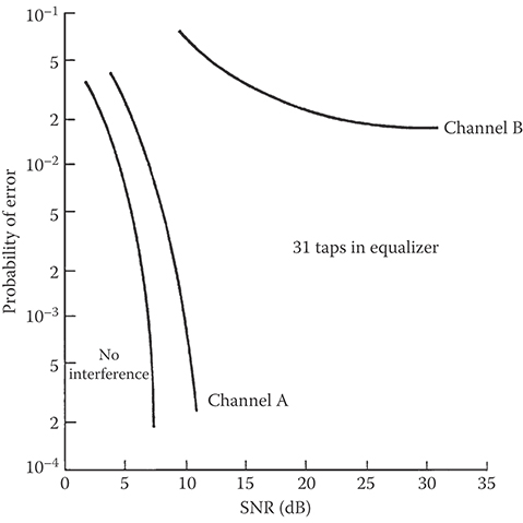
FIGURE 9.18 Error-rate performance of linear MSE equalizer.

A decision-feedback equalizer (DFE) is a nonlinear equalizer that employs previous decisions to eliminate the ISI caused by previously detected symbols on the current symbol to be detected. A simple block diagram for a DFE is shown in Figure 9.19. The DFE consists of two filters. The first filter is called a feedforward filter and it is generally a fractionally spaced FIR filter with adjustable tap coefficients. This filter is identical in form to the linear equalizer already described. Its input is the received filtered signal y(t) sampled at some rate that is a multiple of the symbol rate, for example, at rate 2/T. The second filter is a feedback filter. It is implemented as an FIR filter with symbol-spaced taps having adjustable coefficients. Its input is the set of previously detected symbols. The output of the feedback filter is subtracted from the output of the feedforward filter to form the input to the detector. Thus, we have

z_{m} = \sum_{n = - N_{1}}^{0} c_{n} y (m T - n τ) - \sum_{n = 1}^{N_{2}} b_{n} {\tilde{I}}_{m - n} (9.41)

$z_{m} = \sum_{n = - N_{1}}^{0} c_{n} y (m T - n τ) - \sum_{n = 1}^{N_{2}} b_{n} {\tilde{I}}_{m - n} (9.41)$

where {c_n} and {b_n} are the adjustable coefficients of the feedforward and feedback filters, respectively, Ĩ_m–n, n = 1, 2, …, N₂ are the previously detected symbols, N₁ + 1 is the length of the feedforward filter, and N₂ is the length of the feedback filter. Based on the input z_m, the detector determines which of the possible transmitted symbols is closest in distance to the input signal I_m. Thus, it makes its decision and outputs Ĩ_m. What makes the DFE nonlinear is the nonlinear characteristic of the detector that provides the input to the feedback filter.

Images

FIGURE 9.19 Block diagram of DFE.

Images

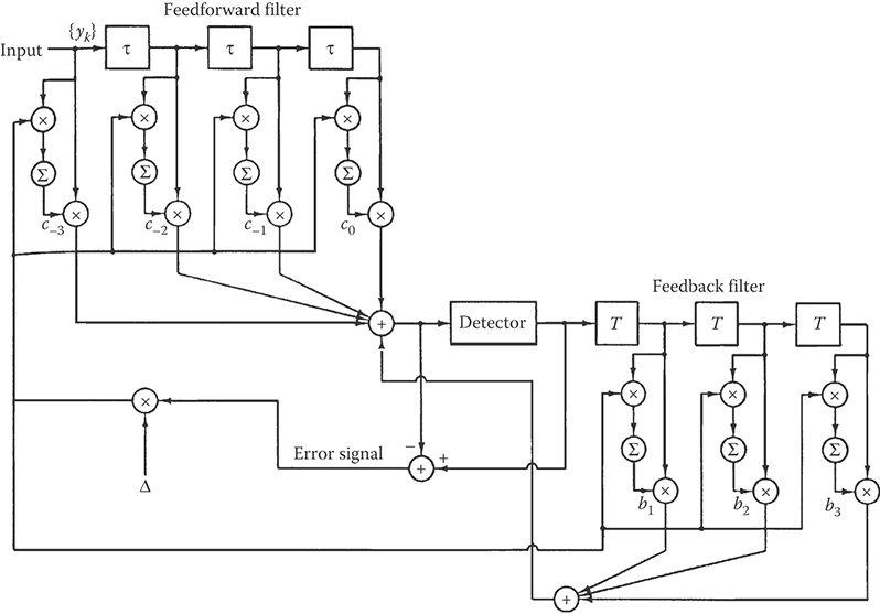
FIGURE 9.20 Adaptive DFE.

The tap coefficients of the feedforward and feedback filters are selected to optimize some desired performance measure. For mathematical simplicity, the MSE criterion is usually applied, and a stochastic gradient algorithm is commonly used to implement an adaptive DFE. Figure 9.20 illustrates the block diagram of an adaptive DFE whose tap coefficients are adjusted by means of the LMS stochastic gradient algorithm. Figure 9.21 illustrates the probability of error performance of the DFE, obtained by computer simulation, for binary PAM transmission over channel B. The gain in performance relative to that of a linear equalizer is clearly evident.

We should mention that decision errors from the detector that are fed to the feedback filter have a small effect on the performance of the DFE. In general, a small loss in performance of one to two decibels is possible at error rates below 10⁻², as illustrated in Figure 9.21, but the decision errors in the feedback filters are not catastrophic.

9.5 Maximum-Likelihood Sequence Detection

Although the DFE outperforms a linear equalizer, it is not the optimum equalizer from the viewpoint of minimizing the probability of error in the detection of the information sequence {I_k} from the received signal samples {y_k} given in Equation 9.5. In a digital communication system that transmits information over a channel that causes ISI, the optimum detector is a maximum-likelihood symbol sequence detector which produces at its output the most probable symbol sequence {Ĩ_k} for the given received sampled sequence {y_k}. That is, the detector finds the sequence {Ĩ_k} that maximizes the likelihood function

Λ ({I_{k}}) = \ln p ({y_{k}}) | {I_{k}}) (9.42)

$Λ ({I_{k}}) = \ln p ({y_{k}}) | {I_{k}}) (9.42)$

Images

FIGURE 9.21 Performance of DFE with and without error propagation.

where p({y_k} | {I_k}) is the joint probability of the received sequence {y_k} conditioned on {I_k}. The sequence of symbols {Ĩ_k} that maximizes this joint conditional probability is called the maximum-likelihood sequence detector.

An algorithm that implements maximum-likelihood sequence detection (MLSD) is the Viterbi algorithm, which was originally devised for decoding convolutional codes. For a description of this algorithm in the context of sequence detection in the presence of ISI, the reader is referred to the paper by Forney [1] and the text by Proakis [4].

Images

FIGURE 9.22 Comparison of performance between MLSE and decision-feedback equalization for channel B of Figure 9.16.

The major drawback of MLSD for channels with ISI is the exponential behavior in computational complexity as a function of the span of the ISI. Consequently, MLSD is practical only for channels where the ISI spans only a few symbols and the ISI is severe, in the sense that it causes a severe degradation in the performance of a linear equalizer or a DFE. For example, Figure 9.22 illustrates the error probability performance of the Viterbi algorithm for a binary PAM signal transmitted through channel B (see Figure 9.16). For purposes of comparison, we also illustrate the probability of error for a DFE. Both results were obtained by computer simulation. We observe that the performance of the maximum-likelihood sequence detector is about 4.5 dB better than that of the DFE at an error probability of 10⁻⁴. Hence, this is one example where the ML sequence detector provides a significant performance gain on a channel with a relatively short ISI span.

9.6 Conclusions

Channel equalizers are widely used in digital communication systems to mitigate the effects of ISI caused by channel distortion. Linear equalizers are widely used for high-speed modems that transmit data over telephone channels. For wireless (radio) transmission, such as in mobile cellular communications and interoffice communications, the multipath propagation of the transmitted signal results in severe ISI. Such channels require more powerful equalizers to combat the severe ISI. The DFE and the MLSD are two nonlinear channel equalizers that are suitable for radio channels with severe ISI.

References

1. Forney, G. D., Jr., Maximum-likelihood sequence estimation of digital sequences in the presence of intersymbol interference. IEEE Trans. Inform. Theory, IT-18, 363–378, 1972.

2. Lucky, R. W., Automatic equalization for digital communications. Bell Syst. Tech. J., 44, 547–588, 1965.

3. Lucky, R. W., Techniques for adaptive equalization of digital communication. Bell Syst. Tech. J., 45, 255–286, 1966.

4. Proakis, J. G., Digital Communications, 4th ed., McGraw-Hill, New York, 2001.

Table of Contents for
9 Channel Equalization

9

Channel Equalization

9.1 Characterization of Channel Distortion

9.2 Characterization of Intersymbol Interference

9.3 Linear Equalizers

Solution

9.3.1 Adaptive Linear Equalizers

9.4 Decision-Feedback Equalizer

9.5 Maximum-Likelihood Sequence Detection

9.6 Conclusions

References

Further Reading

Table of Contents for 9 Channel Equalization

Create new playlist

Sign In

Sign Up

9

Solution

Table of Contents for
9 Channel Equalization