2.1 Introduction

2.2 Frost Forecast Example

2.3 Misclassification Rate

2.4 Sensitivity and Specificity

2.5 Computations Using PROC FREQ

2.1 Introduction

One of the simplest scenarios for prediction is the case of a binary predictor. It is important not only because it contains the most critical building blocks of an ROC curve but also because it is often encountered in practice. This chapter uses an example from weather forecasting to illustrate the concepts. Problems dealing with similar data are abundant as well, ranging from diagnostic medicine to credit scoring.

2.2 Frost Forecast Example

Thornes and Stephenson (2001) reviewed the assessment of predictive accuracy from the perspective of weather forecast products. Their opening example is very simple and accessible to all data analysts regardless of their training in meteorology. The example discusses frost forecasts produced for the M62 motorway between Leeds and Hull in the United Kingdom during the winter of 1995. A frost occurs when the road temperature falls below 0 °C. First, the forecast for each night is produced as a binary indicator (frost or no frost). Then the actual surface temperature of the road is monitored throughout the night and the outcome is recorded as frost if the temperature dropped below 0 °C and as no frost if it did not drop below 0 °C. The guidelines provided by the Highways Agency mandate the reporting of results (both forecast and actual) in a consolidated manner (see the Frost and No Frost columns and rows in Table 2.1) only for the days for which the actual temperature was below 5 °C. The example refers to the winter of 1995, when the actual road surface temperature was below 5 °C on 77 nights. The results are given in Table 2.1. Such a tabular description is the standard way of reporting accuracy when both the prediction and the outcome are binary. It is visually appealing and simple to navigate, and it contains all the necessary information.

There were 29 nights when frost was forecast and a frost was observed, and there were 38 nights when no frost was forecast and no frost was observed. Those two cells (the shaded portion of Table 2.1) represent the two types of correct forecast. A general terminology for these two cells is true positives (TP) and true negatives (TN). The roots of this terminology can be found in medical diagnostic studies when a test is called positive if it shows disease and negative if it does not. By analogy, you can consider frost to mean positive and no frost to mean negative, in which case there are 29 true positives and 38 true negatives in Table 2.1.

Table 2.1 Forecast Accuracy for Road Surface Temperatures

What about forecast errors? There were 6 nights when a frost was forecast and none was observed. There were 4 nights when no frost was forecast, but a frost was observed. One can easily extend the terminology to call these two cells false positives (FP) and false negatives (FN). Table 2.2 is a generic representation of Table 2.1 using the terminology introduced here.

Table 2.2 Reporting Accuracy for Binary Predictions

2.3 Misclassification Rate

There are a variety of ways to summarize forecast accuracy. An obvious one is the misclassification rate (MR), which is the proportion of all misclassified nights, the sum of false negative and false positives, out of all nights:

One minus the misclassification rate is sometimes called percent correct or simply accuracy. The MR for the data in Table 2.1 is 10/77=13%.

While the misclassification rate is simple to compute and understand, it is sometimes too crude for understanding the mechanism behind misclassification. It is also prone to bias if the information is not assembled carefully. Suppose that instead of following the Highways Agency's guidelines, the forecast provider decided to include all nights in a calendar year. There are 77 nights reported in Table 2.1 and, by definition, all those nights the actual temperature dropped below 5 °C. Therefore, the remaining 288 nights were all above 5 °C (no frost), bringing column marginal totals to 33 nights with frost (unchanged) and 332 nights with no frost. It is possible that the MR for the 288 nights when the temperature was above 5 °C was much less than the MR for the nights when the temperature was below 5 °C. Suppose that the misclassification rate for these 288 nights was 5%, resulting in 15 misclassified nights (rounded up). Then there would be a total of 25 misclassified nights out of 365 and the MR would be 25/265=7%. Table 2.3 shows several possibilities.

Table 2.3 Percent Misclassified for the 288 Nights When the Temperature Was above 5 °C and the Corresponding MR for All 365 Nights

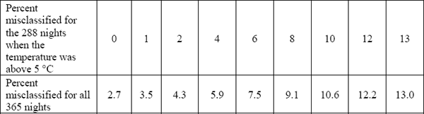
It is clear that the MR is sensitive to which nights are included in the sample because the performance of the forecast is not homogeneous for all the nights in a year. It is also clear that as you include more easy-to-forecast nights in the sample, the MR becomes smaller. You can safely assume that for warm days in spring and summer no nightly frost forecast for the M62 is necessary because most people can make the same prediction (no frost!) quite accurately without resorting to a scientifically obtained forecast. This explains why the Highways Agency restricts the accuracy reporting to nights when the actual temperature was 5 °C or less. It also highlights the fact that interpretation of the MR depends on the proportion of nights with frost in the sample (30% in this example). This proportion is sometimes called prevalence.

In unregulated areas such as credit scoring, where scoring algorithms remain mostly proprietary, there are no such rules, or even guidelines, on how accuracy should be evaluated. In addition, consumers of predictions are not always diligent or knowledgeable in interpreting the details or intricacies of accuracy. Therefore, you need measures that are more robust.

2.4 Sensitivity and Specificity

The most common way of reporting the accuracy of a binary prediction is by using the true (or false) positives and true (or false) negatives separately. This recognizes that a false negative prediction may have different consequences than a false positive one. It also makes these measures independent of prevalence. For this reason, these two measures are considered to gauge the inherent ability of the predictor. In this weather forecast example, a false positive is probably less costly because its primary consequence may be more cautious and better-prepared drivers. On the other hand, a false negative may end up in insufficient preparation and accidents. This suggests reporting false positive and false negative rates separately.

It is more common to work with true positive and true negative rates, defined as

The true positive rate (TPR) is sometimes called sensitivity and the true negative rate (TNR) is sometimes called specificity. While these are generic terms that routinely appear in statistics literature, each field has come up with its own terminology. Weather forecasters, for example, use the miss rate for FNR and the false alarm rate for FPR.

The FNR and FPR for the weather forecast data are 4/33=12% and 6/44 = 14%, respectively. The sensitivity and specificity are 29/33=88% and 38/44=86%, respectively. In this instance, the FPR and FNR are both very close to each other. When this is the case, they will also be very close to the MR. In fact, the MR is a weighted average of the FPR and the FNR: MR = w^*FPR + (1-w)^*FNR, where the weight (w) is the proportion of nights with an observed frost. This is sometimes called the prevalence of frost.

Note that the denominators for TPR and TNR are the total observed positives and negatives. It is possible to define similar quantities using the forecast positives and negatives as the denominator. In this case, the ratios corresponding to sensitivity and specificity are called the positive predictive value (PPV) and negative predictive value (NPV):

SAS users familiar with PROC LOGISTIC recognize that PPV and NPV are actually called TPR and TNR. This may be a source of confusion. This book doesn't use the established PROC LOGISTIC terminology because it defines TPR and TNR consistent with the way they are used in medical diagnostics literature. Nevertheless, to minimize confusion, sensitivity and specificity are used more often than TPR and TNR.

2.5 Computations Using PROC FREQ

It is relatively easy to compute all of these measures in SAS. The following DATA step prepares the data for subsequent use by PROC FREQ:

data m62;
   input forecast $ observed $ weight;
   datalines;
Frost Frost 29
Frost No_Frost 6
No_Frost Frost 4
No_Frost No_Frost 38
;
run;

The following execution of PROC FREQ provides the necessary calculations:

proc freq data=m62;
   table forecast*observed;
   weight weight;
run;

Output 2.1 contains many useful pieces of information. As a quick refresher on PROC FREQ output, the key to the four numbers in each cell is found in the upper left portion of the table. The first number is the frequency (i.e., TP, FP, FN, and TN). The second number (Percent) uses the table sum (the sum of column sums or the sum of row sums, 77 in this example) as the denominator. The third number (Row Pct) is the row percentage (i.e., the proportion that uses row sums as the denominator). Finally, the fourth number (Col Pct) is the column percentage using column sums as the denominator.

Output 2.1

Each of these numbers has a role in computing the measures discussed so far. For example, the MR is the sum of the table percentages (the second set of numbers) in the off-diagonal elements of the table: 7.79+5.19=12.98%. The PPV and NPV can be found among row percentages since row sums pertain to the predictions. Here, the PPV is 82.86% and the NPV is 90.48%. Finally, the sensitivity and specificity are available from the column percentages (87.88% and 86.36% in this example), implying a sensitivity of 87.88% and a specificity of 86.36%.

It is very important to understand the correct interpretation of sensitivity, specificity, PPV, and NPV. Let's start with predictive values first. Their denominators are the number of positive and negative forecasts. In the weather forecast example, the PPV can be interpreted as the probability of an actual frost when a frost is forecast, and the NPV is the probability of observing no frost when no frost is forecast. Hence, if a frost is forecast for the M62 motorway, the probability that there will actually be a frost is estimated to be 82.86%. Similarly, if the forecast does not call for a frost, then the probability that there will be no frost is estimated to be 90.48%.

In contrast, the denominators for sensitivity and specificity are observed positives and negatives. Therefore, sensitivity is the probability that a night with a frost will be correctly identified by the forecast out of all nights with a frost during the winter; similarly, specificity is the probability that a night without a frost will be correctly identified by the forecast out of all nights with no frost (and less than 5 °C) during the winter. In our example, the probability that a frost will be correctly forecast is estimated to be 87.88% and the probability that no frost will be correctly forecast is estimated to be 86.36%.

It is easy to imagine the utility of these probabilities as occasional consumers of a weather forecast. If you drive from Leeds to Hull on the M62 only a few nights during a winter, all you care about is whether the forecast will be accurate on those few nights. On the other hand, the agency responsible for keeping the motorway free of frost might be more interested in sensitivity and specificity when deciding whether to pay for these forecasts since that speaks to the entire “cohort” of nights in the upcoming winter, and the decision of the agency should be based on the performance of the forecast in the long run.

It is easy to recognize that sensitivity, specificity, and positive and negative predictive values are all binomial proportions if the corresponding denominators are considered fixed. The technical term is conditioning on the denominators. This gives easy rise to the use of binomial functionality within PROC FREQ to compute interval estimates.

The following code uses two separate calls to PROC FREQ to obtain estimates of sensitivity and specificity along with confidence intervals and a test of hypothesis about a specific null value. Note the use of the WHERE statement to choose the appropriate denominator for each calculation:

title “Sensitivity”;
proc freq data=m62 (where=(observed= ‘Frost’));
   table forecast / binomial(p=0.8);
   weight weight;
   exact binomial;
run;

The values specified in parentheses following the BINOMIAL keyword are the null values for the test of hypothesis. A null value of 80% is specified. This value is chosen only to demonstrate the hypothesis testing feature of the BINOMIAL option. It does not correspond to an actual value of interest in the example.

Output 2.2 shows the sensitivity, which is estimated to be 87.88% or 29 out of 33. Each of these 33 nights of frost can be thought of as independent Bernoulli variates: 29 of them were positive (1) and 4 were negative (0). Their sum (29) is the binomial variate with a sample size (denominator) of 33, with sensitivity as the binomial proportion of the variate.

Output 2.2

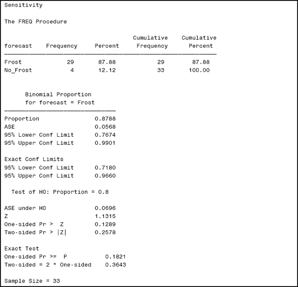
The first set of confidence limits are based on the well-known normal approximation to the binomial. The key quantity for these confidence intervals is the asymptotic standard error (ASE), which is given by

where n is the denominator for the binomial proportion (in this example, sensitivity) and p is the estimate of the proportion from the data. The ASE for sensitivity is 5.68%.

The confidence limits appearing under the ASE are based on asymptotic theory. If n is large, then the 95% confidence interval can be calculated using

p ± 1.96 × ASE

The output reports that the asymptotic 95% confidence interval for sensitivity is (76.74%, 99.01%).

Exact confidence limits, in contrast, are based on the binomial distribution, and they have better coverage in small samples and/or rare events. Because they are calculated by default when the BINOMIAL option is specified, there is no need to use the asymptotic confidence limits. The exact 95% confidence interval for sensitivity is (71.80%, 96.60%). The difference between the asymptotic and exact intervals highlights the typical effects of moderate sample size.

Finally, the last part of the output provides a test of whether the sensitivity is equal to 80% or not. The z-statistic reported in the PROC FREQ output is computed by z = p/ASE(null), where ASE(null) means the ASE under the null hypothesis. This is a typical way of computing test statistics, sometimes referred to as a Wald test. The ASE(null) for our hypothesis is 6.96% and the corresponding z-value is 1.13. In large samples, z has a normal distribution under the null hypothesis so a p-value can be obtained by referring to a standard normal table. This results in a two-sided p-value of 0.26, suggesting that the sensitivity of frost forecast is no different than 80%.

There is an important difference between confidence intervals and hypothesis tests in general regarding the computation of the asymptotic standard error. The ASE of 5.68% uses the observed p of 87.88% while the ASE under H₀ (6.96% here) uses the p of 80% from the null hypothesis.

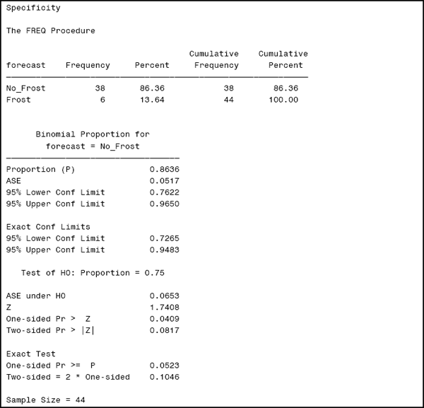
Output 2.3 pertains to specificity.

Output 2.3

The following code creates Output 2.3:

title “Specificity”;
proc freq data=m62(where=(observed=‘No_Frost’)) order=freq;
   table forecast / binomial(p=0.75);
   weight weight;
   exact binomial;
run;

The interpretation of the output for specificity is similar to that of sensitivity. Specificity is estimated to be 86.36% with an ASE of 5.17%. The 95% confidence interval based on the ASE is (76.22%, 96.50%) and the 95% exact confidence interval is (72.65%, 94.83%). A test of whether the specificity exceeds the pre-specified target of 75% yields an asymptotic p-value of 0.0817 and an exact p-value of 0.1046. You would retain the null hypothesis in this case based on this analysis.

The ORDER= option in PROC FREQ may be helpful in situations where SAS, by default, is choosing a binomial event different from the one you want. This leads to the computation of binomial proportions in a way that is the complement of the desired category. You can always subtract the values in the output from 1 and adjust the hypothesized value in a similar fashion to obtain the correct analysis. But it is also possible to obtain exactly the desired output by using the ORDER option of the PROC FREQ statement. To better understand the correct usage of the ORDER statement, it is important to understand that, by default (that is, in the absence of an ORDER option) PROC FREQ uses as event the first value in the alphabetically ordered list of unformatted values of the TABLE variable. This leads to frost being considered an event and the reported analysis is for FPR, not for specificity. ORDER=FREQ tells PROC FREQ to use the category that is most common as the event, leading to the desired analysis. This works when the specificity is greater than 50%, which should cover most cases. When the specificity is less than 50%, then ORDER=FREQ also uses the incorrect category for events. A fail-proof system requires sorting the data first by the predictor variable, in a descending fashion, and then using PROC FREQ without the ORDER= specification.