
ROC Curves with Censored Data |
|

7.3 ROC Curves with Censored Data
7.4 Concordance Probability with Censored Data
7.5 Concordance Probability and the Cox Model
7.1 Introduction
In many applications, the binary outcome event is not immediately observable. For example, most credit scoring algorithms try to predict the probability of default by a certain time. If every subject in the data set is under observation at least until that time, then the outcome is truly binary and the methods we have seen so far are applicable. But it may not be desirable to wait until the outcome for all subjects is observed. It is possible to perform a time-to-event analysis, replacing the yes/no default with time elapsed until default. This analysis has the advantage of accommodating variable follow-up across subjects. Although it is not as powerful as waiting until all subjects reach the pre-specified time, it can usually be accomplished much quicker and the loss in efficiency is usually minimal.
7.2 Lung Cancer Example
Lung cancer is one of the most common and lethal cancers. Its prognosis is heavily influenced by two factors: tumor size and lymph node involvement. Using these factors, you can predict the likelihood of death and plan further treatment accordingly. These factors are best measured on the tumor specimen that is removed during surgery. However, there is considerable interest to accurately characterize the prognosis before surgery. Chapter 3 described the standardized uptake value (SUV) from a positron emission tomography (PET) scan. In this example we will examine the accuracy of SUV as a marker of lung cancer mortality. The goal of this analysis is to see if the SUV can predict survival in lung cancer patients following surgery. Since the SUV is available before surgery, it would have important practical consequences if it has reasonable predictive value.
The data set for this study has three variables: SUV, Survival, and Status. Survival is the time elapsed between surgery and death. For patients who are alive at the time of analysis, it represents the time between surgery and last follow-up. Status is a binary variable indicating whether the patient was dead or alive at last contact. If status = 1, then the patient was dead and the Survival variable is the actual survival time. If status = 0, then the patient was alive and Survival is the follow-up time. These patients are said to be censored because we do not observe their survival time.
This data structure is fairly typical of censored data, and it immediately reveals the intricate features of the required statistical analysis. The outcome (that is, the survival time) is represented by a combination of two variables (Survival and Status) in a specific way. Furthermore, for a subset of the patients, the actual outcome is not observed. Traditional statistical methods cannot be directly applied to the Survival variable for making inferences about survival time. For example, the median of the Survival variable will be an underestimate of the actual median because it treats the follow-up time of censored patients as if it was the actual survival time.
For this reason, analysis of censored data requires special methods. Because censored data are ubiquitous in clinical research, not to mention several other areas such as engineering reliability (time to equipment failure) and finance (time to default), these special methods have been widely studied. This chapter uses two of the more popular censored data methods. One is the Kaplan-Meier estimate of the survival time distribution and the other is the proportional hazards (Cox) regression. We have already made use of the Cox model in the previous chapter, although from a completely different perspective.
Strictly speaking, little prior knowledge about censored data is required to understand this chapter, but it would be difficult to grasp the details without some experience. Paul Allison's Survival Analysis Using the SAS System: A Practical Guide (1995) or Alan Cantor's SAS Survival Analysis Techniques for Medical Research, Second Edition (2003), both SAS Press books, can be helpful for this purpose.
7.3 ROC Curves with Censored Data
We have repeatedly emphasized that generating an ROC curve requires a binary outcome. If W is a predictor and D is the binary outcome, you could write
![]()
to denote the sensitivity and the specificity corresponding to a certain threshold, c. We have seen in Chapter 3 that these two probabilities can be written in terms of the conditional distributions of W and that they form the basis for the empirical ROC curve.
In the context of survival models, the outcome is the time elapsed until an event (such as death or default) takes place. This can be viewed as a binary outcome as a function of time. Equation (7.1) is now replaced by
![]()
which highlights the fact that sensitivity and specificity are functions of time in the context of censored data.
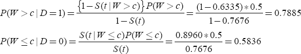
Using Equation (7.2), we can estimate the sensitivity and specificity for each c and plot these estimates to get the ROC curve at a specific time point, t. The estimates can be obtained using the following relations, which follow from the definition of conditional probability as well as application of the Bayes theorem:

In Equation (7.3) and elsewhere in this chapter, S(t) denotes the survival function—that is, S(t)=P(T>t). It turns out that the three components on the right-hand side of Equation (7.3) can all be calculated using SAS. The following sections detail how Equation (7.3) can be computed using the data. For illustration, we will use c=9 and t=36, but the following steps can be repeated for other values of c and t as well.
7.3.1 Estimation of S(t)
As noted previously, S(t)=P(T>t) is the survival function of the variable T (one minus the familiar cumulative distribution function), which is subject to censoring. Computing the cumulative distribution of a censored variable requires special methods. The most popular of these methods, alternatively known as the Kaplan-Meier or product limit method of estimation, is implemented in PROC LIFETEST in SAS/STAT software. PROC LIFETEST is the primary vehicle to compute the distributions required when using Equation (7.3). The following call returns the probability of survival at 3 years:
The TIME statement has a special syntax, which combines information about the outcome from the two columns. The variable specified first (before the asterisk) is the survival time, and the variable specified second (after the asterisk) is the status. In parentheses after the status variable is a list of values that identify which values of the status variable indicate censoring. Finally, timelist=(36) prints out only the 3-year (36-month) estimates of the survival function. Otherwise, by default, survival probabilities for all time points observed in the data set are printed.
Output 7.1 shows the results of this invocation of PROC LIFETEST. The relevant portion is labeled Product-Limit Survival Estimates (product-limit is another name for the Kaplan-Meier estimate). The time point of interest is listed under the heading Timelist and the corresponding probability is labeled as Survival. Remember that S(t)=P(T>t) and also note that 1−S(t)=P(T<t) is given under the Failure heading. We see from the results in Output 7.1 that S(t)=0.7676 and 1−S(t)=0.2324.
Output 7.1

7.3.2 Estimation of P(T|W)
P(T|W) is also, fundamentally, a time-to-event distribution and can again be estimated with PROC LIFETEST. The key point to remember is to exclude the appropriate patients based on the condition specified in W. Hence, when you compute P(T|W>9), you need to include only those patients with an SUVgreater than 9, as shown in the following call to PROC LIFETEST:
Output 7.2, which has the same format as Output 7.1 (with only the relevant portions shown), informs us that 1−S(T|W>9)=0.3665. The equation S(T|W≤9), obtained similarly (though not shown here), equals 0.8960.
Output 7.2

7.3.3 Estimation of P(W)
W is not subject to censoring, so, in principle, P(W>c) is the proportion of observations exceeding c. P(W) can be computed in many different ways in SAS, including using a DATA step or PROC SQL programming as well as using PROC UNIVARIATE and PROC FREQ. You can also use PROC LIFETEST because, in the absence of censoring, Kaplan-Meier methods produce the same results that would have been obtained from the standard methods. Because specifying a status variable is optional, PROC LIFETEST can be used for this purpose, as follows:
This is a somewhat unusual call after the previous PROC LIFETEST calls. SUV is the variable for which a distribution is needed; hence, timelist=9. The lack of a status variable is due to the fact that W is not subject to censoring. The output from PROC LIFETEST (Output 7.3) indicates that P(W>9)=0.50. This is also the first example where the values under the headings Timelist and SUV differ. The former lists the value(s) requested by the TIMELIST= option of the PROC LIFETEST statement and the latter shows the nearest observed value for which the reported survival and failure probabilities hold. If the requested time point is observed, then the two columns will have identical numbers.
Output 7.3

7.3.4 Putting It Together
Sections 7.3.1 through 7.3.3 demonstrate how the components of Equation (7.3) can be computed from the data using the SAS procedure PROC LIFETEST. Using the results of these sections, you can compute the sensitivity and specificity for an SUV of 9 at 3 years as follows:
By varying c, you can obtain the sensitivity and one minus specificity for each c. A plot of these pairs constitutes the ROC curve.
There is a potential problem here, however. In the examples presented in Chapter 3, the ROC curve was guaranteed to be monotone-increasing. There is no such guarantee for censored data because Kaplan-Meier estimates are not smooth functions of time (they have several jumps). This implies that, as one minus specificity increases, sensitivity might occasionally decrease, violating a central premise of the ROC curve. Lack of monotonicity may be obvious in small samples, but in most data sets with large samples and/or events, it is hardly noticeable.
If the estimate of S(t) had no jumps and flat regions—that is, if it were monotone itself—the ROC curve would also have been monotone. Realizing this, Heagerty et al. (2000) suggest a different estimator for S(t), a weighted Kaplan-Meier estimator.
The macro %TDROC generates a time-dependent ROC curve. The required inputs to the macro are DSN (the data set name), Marker, TimeVar, Status, and TimePT. The TimePT variable specifies the time at which predictions are to be made. The Status variable must satisfy the requirements of PROC LIFETEST: It must be numeric and it must be followed, in parentheses, by the list of values that indicate censoring. The macro also has an option (smooth=1) that implements a smooth estimator of S(t). By default, smooth=0. Another optional input is PLOT (by default, 1), which controls whether the curve is plotted. When plot=0, only data sets with pairs of sensitivity and specificity are made available.
Figure 7.1 is an ROC curve for SUV as a marker of prognosis at 3 years using the lung cancer data generated by the following call to the %TDROC macro:
Figure 7.1 The ROC Curve at 3 Years for the Predictive Power of SUV in Lung Cancer

The AUC for the ROC curve in Figure 7.1 is 0.657 and suggests a moderate level of accuracy. The curve itself is never too far from the diagonal line, supporting the same conclusion. Of course, the ROC curve should be evaluated in the context of competing methods of prediction. In survival analysis, making accurate predictions is much more difficult because the event being predicted, in some cases, is several years away, during which many other things can happen to the patient. From this perspective, an AUC of 0.657 represents a respectable level of accuracy.
It is obvious that the choice of time point can influence the conclusions. In some cases, investigators have a clear target time point. Other studies lack such clarity and may pose a problem to the statistician in choosing the time point. In these cases, try out a few time points and present the results simultaneously, as in Figure 7.2.
Figure 7.2 The ROC Curves at 2, 3, and 4 Years for the Predictive Power of SUV in Lung Cancer

To generate a display like Figure 7.2, you need to understand how the output data sets are named by the %TDROC macro. The data set name in macro language is &&DSN_&TIMEPT, so for the lung cancer example, the data sets for the three ROC curves in Figure 7.2 are named LUNG_24, LUNG_36, and LUNG_48.
In general, the three curves have similar shapes, although sensitivity seems to increase with time at high levels of specificity and decrease with time at low levels of specificity. The AUCs of the three curves are 0.618, 0.657, and 0.729, suggesting that the SUV is better able to predict the status of patients at later years than earlier years. On the other hand, most of the difference between the curves is in the region where specificity is less than 0.5 and hence the difference in AUCs may be immaterial from a practical perspective.
7.4 Concordance Probability with Censored Data
Section 7.3 explained how to construct ROC curves with censored data. The principle idea is to dichotomize the time-to-event outcome at a given time point. As a result, the ROC curve is defined for a specific point in time. To get an idea about the overall predictive value of a marker, you need to perform an analysis like the one presented in Figure 7.2.
This section discusses an alternative method to assess the overall value of a marker in predicting a censored outcome. This alternative approach is based on the idea of concordance. In Chapter 3, we saw that, for a binary outcome, the area under the empirical ROC curve is equivalent to the concordance probability. As a reminder, the concordance probability is defined on a pair of subjects where one of the pair has the outcome and the other does not. The probability that the subject with the outcome has a greater marker value than the other subject is called the concordance probability.
The following way to express concordance probability is consistent with this definition and also makes it amenable to extend this definition to censored outcomes. Define
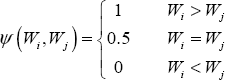
Hence ψ indicates which member of the pair has the higher value, with ties indicated by 0.5. Suppose there are n patients with the outcome and m patients without the outcome. Then, there are a total of mn pairs and the concordance probability can be written as follows:
![]()
The summation represents the number of pairs that have Wi>Wj (with an accommodation for ties), so the entire expression is the fraction of patient pairs where the one with the higher marker value had the outcome.
You can use the idea of concordance in time-to-event settings. To see how the definition of concordance can be adopted for censored outcomes, let Ti and Tj be the event times in a given pair of patients with marker values W1 and W2. The concordance between a marker W and the censored outcome T is defined as
![]()
Because T is subject to censoring, this estimator cannot be used since the outcome is partially observed.
Harrell et al. (1982) suggest a modification of this estimator that can be used with censored data. This method is based on the realization that even in the presence of censoring, the outcome in some of the pairs can be ordered. For example, if the second subject is dead with a survival time that is shorter than the follow-up time of the first subject who is alive, we can say with certainty that T1>T2. Table 7.1 lists all the possibilities and the corresponding value of ψ (W1,W2). If Ψ (W1,W2)=1, it indicates that the prediction and the outcome are concordant. If Ψ (W1,W2)=0, it indicates that the prediction and the outcome are discordant. Finally, (W1,W2)=? means that, due to censoring, it is not possible to determine whether the prediction and the outcome are concordant or discordant.
Table 7.1 All Possible Pairings and Concordance Status with Censored Data

Now we can evaluate all the pairs to see whether they are concordant or not using the definitions in Table 1. The denominator is the number of informative pairs (that is the pairs for which we can make a decision), indicated in the following equation by k. The notation (i,j)=1 to (i,j)=k means that the summation is over pairs of (i,j) and there are k such pairs. The resulting estimator of concordance probability is often called the c-index.
![]()
The c-index has several advantages. It mimics the computation of the area under the ROC curve with binary data, it is intuitive, and it is conceptually simple to compute. Despite the conceptual simplicity, the computation requires forming all pairs and can take a long time. Computation of the c-index is not built into existing SAS procedures, but the %CINDEX macro, available from this book's Web site, can be used to compute it, as follows:
Here, DSN is the name of the data set, Pred is the variable in the data set to be used as the predictor, Surv is the survival time variable, and Cens is the censoring indicator (1 for censored, 0 for event). Output 7.4 simply reports the c-index.
Output 7.4

In the case of the lung cancer example, the concordance probability is estimated to be 0.69, using the c-index as the estimator.
If the question of interest centers around multiple markers or a multivariable predictive model, then the input macro variable PRED of the %CINDEX macro should point to the variable containing the predictions of the multivariate model.
Despite all its advantages, the c-index has one big drawback. It is not a consistent estimator of the true concordance probability. A consistent estimate gets closer to the true value as the sample size increases. However, the c-index can remain far away from the true value even as the sample size increases. Therefore, the c-index can give “wrong” answers even in large samples. In my experience, if the censoring rate is low (which implies that the proportion of undecided pairs is low), the c-index works reasonably well. As the censoring rate increases, its performance becomes unpredictable.
The reason for the inconsistency of the c-index, at least intuitively, is that it uses the observed survival or follow-up times. Unless a parametric model is adopted, procedures using the observed values do not provide consistent estimates. For this reason, most of the non-parametric or semi-parametric methods of analyzing censored data, such as the Kaplan-Meier estimate or the proportional hazards regression, use the ranks of the data, not their actual values.
Before we finish this section, note an interesting property of the concordance probability:
CP(W, T) = 1 – CP(–W, T)
This equation tells us that if a marker is known to have high values when the outcome is unlikely, then CP can be less than 0.5. The more informative measure in this case is 1−CP, which can be taken as a measure of the marker to correctly order event times.
7.5 Concordance Probability and the Cox Model
There is an alternative way of computing the concordance probability in a very important special case. Most cases involving regression with censored data, such as modeling the relationship between a continuous covariate and a censored outcome or between multiple covariates and a censored outcome, are handled within the framework of the Cox model (proportional hazards regression). It turns out that concordance probability can be computed analytically in the context of the Cox model. The following development is from Gönen and Heller (2005).
The starting point is the definition of concordance probability for a censored outcome, as used in Section 7.4:
![]()
where T is the survival time and W is the predictor. For the time being, we will work with a single predictor. Extension to the case of multiple predictors will follow. The Cox model for this case stipulates that
![]()
where h(t) is the hazard function for t, which is written as a product of two terms: one involving t only (h0, the baseline hazard) and one involving W only (the linear part). Using the relationship between hazard and survival functions, you can write the equivalent expression:
![]()
More information on how to show the equivalence of these two expressions can be found in most books covering the Cox model, such as Survival Analysis Using the SAS System: A Practical Guide (Allison, 1995).
Now you can rewrite the concordance probability in terms of survival functions:
![]()
Understanding this equation requires some familiarity with advanced probability, but here it is used to show that concordance probability can be written using only S(t). If you substitute the form of S1 and S2 from the Cox model, then the integral on the righthand side can be evaluated as follows:
![]()
Hence, to evaluate the discriminatory power of the predictor W in the context of a Cox model, you need an estimate of β and the values of W for all possible pairings of the data. Note that T enters the computation only through the estimation of β, which can be accomplished using partial likelihood. Therefore, censoring is naturally handled by the existing methods of fitting a Cox model. This is a particular strength of this approach to computing the concordance probability.
If there are multiple predictors, then both W and β will be vectors. The same expression can be written in vector notation as follows:
![]()
The expressions derived so far involve a particular pair of observations, denoted as 1 and 2. To use this in a set of data involving several observations, we need to compute this probability for each pair of observations. This yields the following formula for an estimate of the concordance probability (labeled CPE for concordance probability estimate):
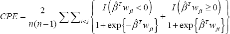
where wji = wj − wi. The summand consists of two parts, representing the case whether higher or lower values of the predictor correlates with longer survival, which is reflected in the sign of the regression coefficient. If β > 0, then higher values of the covariate are associated with higher values of hazard. In this case, if, for a particular pair, wj > wi, then the probability of Tj being greater than Ti should be more than 0.5 and hence the second term of the summand should be applicable since βTWji > 0 and exp{βTji} > 0. Thus, (1+ exp{ βTji})-1 > 0.5. The other three cases depending on the sign of β and wji can be explained in a similar fashion.
As mentioned previously, the availability of Cox model software using partial likelihood is the primary operational advantage. It also constitutes one of the theoretical advantages. Partial likelihood estimates are consistent; that is, as the sample size grows, the results get nearer and nearer the underlying true but unknown value of the parameters. It is well-known that functions of consistent estimators are also consistent. Since β is the only parameter estimated to compute the CPE, it turns out that CPE is also consistent. This is an important reason why you should favor CPE over the c-index in the context of Cox models.
CPE can be estimated using the %CPE macro, which is available from this book's companion Web site at support.sas.com/gonen. The macro call is similar to that of %CINDEX:
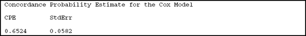
Output 7.5 shows the results.
Output 7.5
An important difference in the macro calls of CINDEX and CPE is that the predictors are listed with blanks in between as if they appeared on the right-hand side of the MODEL statement.
We see that the CPE for the lung data set is less than the c-index. This is usually the case, in my experience. The c-index seems to overestimate the true concordance probability, especially if the censoring proportion in high. Since the CPE is a consistent estimate and the c-index is not (as explained earlier), the CPE is a better measure in the context of using predictions from Cox regression models.