4.1 Introduction

4.2 An Example from Prostate Cancer Prognosis

4.3 Paired versus Unpaired Comparisons

4.4 Comparing the Areas under the Empirical ROC Curves

4.5 Comparing the Binormal ROC Curves

4.6 Discrepancy between Binormal and Empirical ROC Curves

4.7 Bootstrap Confidence Intervals for the Difference in the Area under the Empirical ROC Curve

4.8 Covariate Adjustment for ROC Curves

4.9 Regression Model for the Binormal ROC Curve

4.1 Introduction

In many instances there will be a set of competing predictions to choose from and hence it is often of interest to compare predictions. For example, how does an expensive invasive procedure or radiological scan compare with a simple clinical exam to diagnose a medical condition? Or, is it worth it to obtain at substantial cost detailed credit reports while one already has a simple financial summary of the debtors. Does the incremental increase in accuracy justify the additional cost? The term cost here is used loosely; for example, the additional burden on a patient of performing an additional diagnostic scan is considered a cost. Of course, there are traditional costs to consider, too: The monetary cost of obtaining the additional scan needs to be taken into account as well. Before deciding whether these costs are justified, you need to evaluate the gains in predictive accuracy.

A common and simple way to compare competing predictors is to construct an ROC curve for each one. Visual comparisons of these ROC curves usually reveal several useful features. In addition, two ROC curves can be compared for statistically significant differences. This chapter discusses non-parametric and parametric methods of statistically comparing two or more ROC curves.

4.2 An Example from Prostate Cancer Prognosis

Chapter 3 used an example from cancer diagnosis and monitoring to introduce ROC curves. This chapter uses an example from cancer prognosis to study the methods of comparing two ROC curves. This time, the data are obtained on prostate cancer patients with bone metastases. Traditionally, these patients undergo a bone scan, a radiographic exam that reveals the abnormalities in the bone. You can compute a summary measure, called a bone scan index (BSI), which indicates the extent of bone disease in patients. A competing marker is the SUV from a PET scan that was used in Chapter 3 to identify head and neck cancer. The prostate data set contains measurements of BSI and SUV for 51 patients. The outcome of interest is one-year survival—that is, whether patients are alive one year after their BSI and SUV are measured. Each patient was followed at least one year and the outcome recorded. Forty patients were dead, and 11 were alive at the one-year mark.

This example is used throughout the chapter to compare the ROC curve of SUV with the ROC curve of BSI. But before further discussion, we need to distinguish between paired and unpaired mechanisms of data collection, an important issue associated with most data sets involving ROC curve comparisons.

4.3 Paired versus Unpaired Comparisons

When dealing with any statistical comparison, you need to distinguish unpaired and paired data. Here, unpaired refers to when data in the two groups to be compared are obtained from different sampling units and paired refers to when each sampling unit contributed exactly a pair of observations: one to each group.

Consider the example of a randomized clinical trial that evaluates screening mammography. Women are randomized to either the standard of care, which is periodic clinical exams, or to mammography, which is mammography in addition to the standard of care. The resulting comparison, whether performed using ROC curves or not, is unpaired. Each woman in the study is either in one study arm or the other.

Now, consider another study that evaluates PET in imaging tumors before surgery. Suppose that there is a standard imaging tool for this purpose, likely computed tomography (CT) for most cases. One possibility is randomizing the patients to receive either a CT or a PET, creating an unpaired comparison. However, a statistically more efficient way of comparing the two is arranging for the patients to undergo both scans, creating a paired data situation.

In traditional statistics, most comparisons involve unpaired data as opposed to paired data. For example, the two-sample (unpaired) t-test is probably the most widely applied statistical test. The reason for this is not increased efficiency. In fact, for a fixed sample size, paired techniques are usually more powerful than unpaired ones. It is, however, more difficult, or sometimes impossible, to implement a paired design. Randomized trials of many drugs and interventions use unpaired designs because exposing the subject to multiple treatments or interventions is often difficult, if not impossible. Imagine a trial comparing surgical treatment against watchful waiting, a common option, for early stage indolent tumors such as some cancers of the prostate. It is not possible for patients to undergo both treatments.

Paired comparisons have made their mark as the design of choice in some fields, including comparison of predictive markers. Many of the markers under consideration can be applied to each sampling unit without too much burden, cost, or undue consequence. Thus, this chapter focuses on comparing ROC curves with paired data, although references to unpaired comparisons will be noted.

4.4 Comparing the Areas under the Empirical ROC Curves

In addition to the distinction between paired and unpaired data, you also need to decide what comparing the ROC curves means. It could refer to comparing the curves in their entirety, or it could refer to comparing certain summary measures, such as the area under the curves.

When dealing with empirical ROC curves, the usual choice is comparing the summary measures. The alternative, comparing entire curves, is a difficult task without the help of a model. The caveat, of course, is that two predictors may have the same AUC but very different ROC curves. For this reason, a graphical display of the ROC curves under comparison should always accompany the statistical test comparing the AUCs.

4.4.1 Comparisons with Paired Data

You can organize the paired data in two ways. The most intuitive way is to have one row for each subject and one column for each marker in addition to a column for the outcome. An equivalent way is to have one row for each subject-marker combination, resulting in two rows per subject. The outcome variable will be duplicated in these two rows and an additional column containing the subject identifier will be added to keep track of the pairing. These two data structures are known as wide and long, respectively, with obvious reference to the shape of the data matrix. One can be converted to the other with simple DATA step instructions.

The %ROC macro that was used in Chapter 3 to obtain estimates of the standard error of the AUC can also be used to compare two ROC curves only if the data are paired. The methodology implemented in this macro is essentially non-parametric. Each AUC is estimated using the concordance method described in the previous chapter. The concordance statistic is a member of the class of U-statistics. The variance of the AUCs as well as the covariance between them can be computed using the general principles of the theory of U-statistics. See DeLong et al. (1988) for more information.

The %ROC macro expects the data in the wide form. The following macro call performs the needed comparison:

%roc(data=bone, var=bsi suv1, response=gold, contrast=1 –1);

The VAR macro variable specifies the names of the variables containing the two marker values. The CONTRAST macro variable expects input similar to the CONTRAST statement in PROC GLM, so 1 –1 refers to the difference of the two variables stated in the VAR macro variable.

Output 4.1 shows the results of this call. The AUC estimates for each of the ROC curves, along with their standard errors and (marginal) confidence intervals, appear first. BSI has an AUC of 0.7795, which compares favorably with that of SUV at 0.6773. The standard errors are quite large, however: 0.0771 for BSI and 0.0836 for SUV, resulting in wide confidence intervals. The AUC for BSI has a 95% confidence interval that ranges from 0.6284 to 0.9307. The confidence interval for SUV is between 0.5134 and 0.8412. It seems that SUV is barely distinguishable from a random predictor (since the lower confidence limit barely exceeds 0.50).

Output 4.1

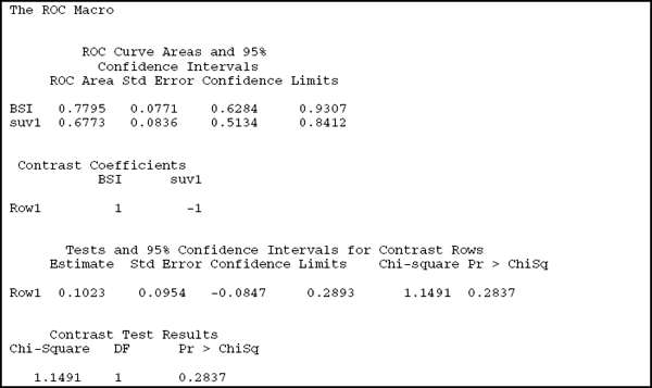
Contrast information appears next. This can be used to verify that the results are for the intended comparison and to infer the direction of the difference. In this example, a positive difference in AUC curves points to BSI being the better test. The next piece of output compares the two ROC curves. The difference in the two AUCs is 0.1023, as reported under the Estimate column. This could be obtained directly as the difference between 0.7795 and 0.6773, the AUCs for BSI and SUV reported in the first part of the output. However, you can not compute the standard error of the difference from the information about the individual areas because the data are paired. Based on this standard error, the difference between the two AUCs is not significant (p=0.2837) and the confidence interval of (–0.0847, 0.2893) spans 0.

It appears that the test statistic and the p-value are reported twice. Had the contrast involved more than one row, then the output on contrast rows would have included one line for each row in the contrast. The part labeled “Contrast Test Results” would still report a single p-value with r–1 degrees of freedom, where r is the number of rows. Therefore, only in a contrast with a single row does information in the “Contrast Rows” section and the “Contrast Test” section coincide.

As discussed here, it is essential to present a visual display of the ROC curves along with the comparison of the AUCs. Figure 4.1 is generated by the %PLOTROC macro introduced in Chapter 3. The syntax modification is similar to the one in the %ROC macro (that is, multiple markers are specified in the VAR macro variable, separated by blanks).

%plotroc (bone bsi,suv,gold,anno=4,tlist1=1.08 2.29, tlist2=4.8 5.8);

Figure 4.1 ROC Curves for BSI (Solid) and SUV (Dashed) Overlaid

Figure 4.1 shows that the BSI has a higher sensitivity than the SUV for most values of the specificity. In the range where sensitivity is 50% through 80%, the sensitivity of BSI is substantially higher than that of SUV. A threshold of 2.29 for the BSI achieves a sensitivity of more than 80% and a specificity of more than 70%. None of the operating points for the SUV offers comparable accuracy. Despite this, keep in mind that the AUC estimates displayed high variability and the difference was not statistically significant.

4.4.2 Comparisons with Unpaired Data

In theory, the %ROC macro can only compare the AUCs of two predictors if the data are paired. Because unpaired designs are so uncommon in the field of ROC curves, no macro performs the desired comparison. Fortunately, unpaired comparisons are easy to be performed by hand or by a few lines of DATA step code: If AUC₁ and AUC₂ are the two AUC estimates with associated standard errors s₁ and s₂, then the test statistic for the unpaired comparison is as follows:

In a large sample, T will have a chi-square distribution with one degree of freedom under the null hypothesis (that is, when the two AUCs are indeed equal).

Note that AUC₁ and s₁ are reported when the %ROC macro is executed for the first predictor only, as explained in Chapter 3. Similarly, AUC₂ and s₂ are estimated from a second %ROC call. Once T is computed, the two-sided p-value can be found using the following line in a DATA step:

p_value=1–probchi(t_unpaired, 1);

If the prostate cancer study offered either a PET or a BSI (but not both) so that the resulting data structure was unpaired, and if the AUC estimates and their standard errors were the same as described previously (0.7795 and 0.6773 for the AUCs, 0.0771 and 0.0836 for the standard errors), then T would be 0.8095 and the p-value would be 0.3683. The increase in p-value using the unpaired design can be explained by the increased efficiency of the paired design, as briefly discussed in Section 4.3.

4.5 Comparing the Binormal ROC Curves

Chapter 3 shows that you can achieve a model-based estimate of the ROC curve by assuming that the distributions of the marker for the diseased and non-diseased groups have normal distributions with possibly different parameters. Specifically, if diseased patients' marker values follow a normal distribution with mean µ₁ and variance σ₁² and if non-diseased patients' marker values follow a normal distribution with mean µ₀ and variance σ₀², then the ROC curve can functionally be written as

with the AUC given by

where the binormal parameters a and b are given by

Next, we discuss paired data in detail; comments about unpaired data appear at the end of this section.

4.5.1 Comparisons Based on the Binormal Model with Paired Data

The paired nature of the data requires some adjustment to the model before you can proceed. Let X_ij denote the marker value for the i^th patient and the j^th marker. Then X_ij (or some transformation of it) is assumed to have the following normal distribution if the patient has a positive outcome:

If the patient has a negative outcome, then X_ij would be distributed as

The u_i is normally distributed as well:

with the key assumption that u_i and u_i, are independent for i≠i'.

This model has four fundamental parameters for each marker: µ_1i and µ_0i are the means of the outcome positive and outcome negative patients for marker j, and σ_1i and σ_0i. are the two standard deviations. In this respect, it is a standard binormal model for each marker separately. To take into account the correlation between the two marker measurements on the same subject, a random effect u is introduced. Because u_i is a subject-specific effect, the two marker values that are measured on the same patient will have the same u_i. This commonality induces a correlation on the two measurements (one for each marker) taken on the same subject. Because u_i and u_i, are independent for i≠i', there is no correlation between marker values that were not measured on the same subject. Use of random effects to induce correlations on selected pairs of subjects is a standard technique in most settings.

The following code segment first runs PROC TRANSREG to identify a transformation to normality. See Section 3.7 for a detailed explanation of the role of this step in fitting binormal models.

proc transreg data=bone;
   model boxcox(suv1/parameter=0.1 geometricmean)=class(gold);
   output out=trsuv;
run;

proc transreg data=bone;
   model boxcox(bsi/parameter=0.1 geometricmean)=class(gold);
   output out=trbsi;
run;

The Box-Cox model identifies the logarithmic transformation for the BSI and the square-root transformation for the SUV as the best possible transformations to normality (detailed PROC TRANSREG output not shown). The output data sets TRSUV and TRBSI are created by the OUTPUT statement in PROC TRANSREG and include the transformed covariates, TBSI and TSUV. These two data sets are combined to form Long, a data set in long form. Then PROC NLMIXED finds the maximum likelihood estimates for the random-effects binormal model, as specified previously.

data long;
   set trbsi(keep=_name_ gold tbsi rename=(tbsi=result _name_=subid)
       in=in1)
   trsuv(keep=_name_ gold tsuv rename=(tsuv=result _name_=subid)
       in=in2);
     if in1 then marker=0; else if in2 then marker=1;
run;

proc nlmixed data=long method=firo technique=quanew;
   parms sr=1 s11=3 s10=0.3 s01=2 s00=0.2 m11=7 m10=1 m01=2 m00=0;
   bounds sr s11 s10 s01 s00>0;
   if gold=1 and marker=0 then do;
             m=m10+u;s=s10**2;end;
   if gold=1 and marker=1 then do;
             m=m11+u;s=s11**2;end;
   if gold=0 and marker=0 then do;
             m=m00+u;s=s00**2;end;
   if gold=0 and marker=1 then do;
             m=m01+u;s=s01**2;end;
   a1=(m11-m01)/s11;
   b1=s01/s11;
   a0=(m10-m00)/s10;
   b0=s00/s10;
   auc1=probnorm(a1/sqrt(1+b1**2));
   auc0=probnorm(a0/sqrt(1+b0**2));
   model result ~ normal(m,s);
   random u ~ normal(0,sr) subject=subid;
   estimate ‘a1’ a1;
   estimate ‘b1’ b1;
   estimate ‘AUC1’ auc1;
   estimate ‘a0’ a0;
   estimate ‘b0’ b0;
   estimate ‘AUC0’ auc0;
   estimate ‘AUC1-AUC0’ auc1-auc0;
   contrast ‘AUC1-AUC0’ auc1-auc0;
   contrast ‘Equality of ROC curves’ a1-a0, b1-b0;
run;

The fundamental description of the model in PROC NLMIXED is similar to the one in Section 3.6, with two exceptions of the random effect u. The RANDOM statement declares u as the random effect. For those familiar with PROC MIXED, the RANDOM statement has similar functionality but different syntax. In PROC MIXED, you don't need to specify the distribution of the random effect since normal random effects are the only available option. In PROC NLMIXED, you must specify the distribution of the random effects since any of the built-in distributions that PROC NLMIXED recognizes is an option. Another difference is that, in PROC MIXED, specifying the RANDOM statement ensures that the random effect is added to the model; in PROC NLMIXED, you must add the term u to the mean function in programming statements. See the appendix for a brief introduction to the syntax and capabilities of PROC NLMIXED.

In addition to the presence of the random effect, this call to PROC NLMIXED is different from the ones in Chapter 3 in a few other ways. For example, the CONTRAST statement provides simultaneous testing of parameters. It is helpful to think of it as multiple ESTIMATE statements executed simultaneously. To make this point, note that

estimate ‘AUC1-AUC0’ auc1-auc0;

and

contrast ‘AUC1-AUC0’ auc1-auc0;

perform the same test (that is, the equality of the AUCs). You would normally do this by using the ESTIMATE statement; including the CONTRAST statement for this purpose is for demonstration only.

The more important use of the CONTRAST statement here is to test the equality of the two ROC curves in their entirety. Note that two binormal ROC curves are identical only if they have the same binormal parameters. Therefore, comparing a and b for two or more binormal curves offers one way of testing whether the two curves are identical. This is accomplished by the following CONTRAST statement:

contrast ‘Equality of ROC curves’ a1-a0, b1-b0;

which tests the null hypothesis

H₀ : a₀ = a₁ & b₀ = b₁

against the alternative that at least one of the binormal parameters is different. Note that it is not possible to express this using an ESTIMATE statement.

Output 4.2 shows the relevant portion of the output.

Output 4.2

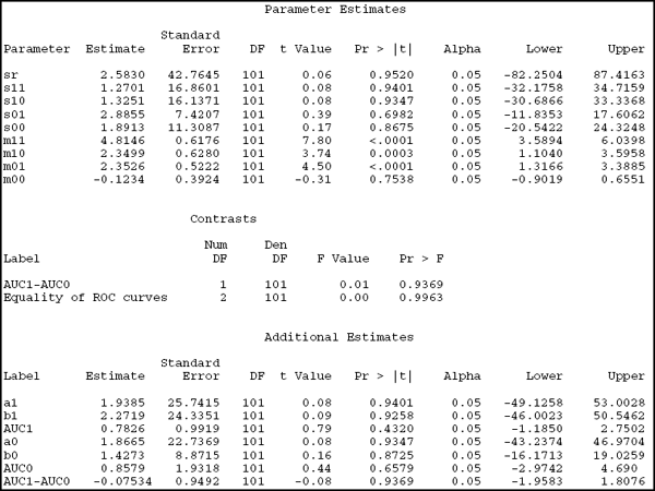
The Parameter Estimates section of the output presents estimates of the model parameters and is of little use here. The more interesting part for ROC analysis is the Additional Estimates section, which provides information on the results of the ESTIMATE statement, including binormal parameters of BSI (a₀ and b₀) and SUV (a₁ and b₁). This section also reports the implied AUC (AUC₁ and AUC₀) for each marker and the difference between the two AUCs. We see that the AUCs are estimated to be 0.7825 for the SUV and 0.8579 for the BSI. Their difference is 0.0753 and is not significant, with p=0.9369.

The two contrasts are reported in the Contrasts section. The first one is the difference between the two AUCs, repeated here only to highlight the similarities between the ESTIMATE and CONTRAST statements. This contrast has the same p-value as the ESTIMATE statement (as it should) but uses the F-statistics rather than t-statistics. If you are familiar with analysis of variance, you will remember that an F-statistic with a single numerator degree of freedom is identical to the square of the corresponding t-statistic. The same principle applies here, although it is hard to see from this output since the test statistics have very small absolute values. Nevertheless, note that t=–0.08, the square of which is 0.01 when rounded to two decimal places.

The contrast of real interest is the simultaneous test of the equality of the two binormal parameters. The results strongly suggest that there is no evidence against the equal ROC curves hypotheses (p=0.99).

4.5.2 Comparisons Based on the Binormal Model with Unpaired Data

As explained in Section 4.5.1, the random effect u was introduced to the binormal model only to account for the within-subject correlation. In unpaired designs, the within-subject correlation is 0 by definition. This suggests a simple way to modify the code from the previous section: Remove u. This amounts to removing the RANDOM statement and cleaning up the way m is defined in the programming statements.

4.6 Discrepancy between Binormal and Empirical ROC Curves

It is not uncommon for the binormal model and the empirical model to reach different conclusions. The difference between them is similar to the difference between rank tests and t-tests. If the assumptions underlying the binormal model are true, then the binormal model has more power, which might explain the significant result. On the other hand, if the model assumptions are not true, then the Type I error may be inflated, which would appear as increased false positive results. Although it is not possible to conclude which one is the driving force, certain features of the PROC NLMIXED output, along with exploratory graphical analyses like the one in Figure 4.2, remain the best way of checking the assumptions of binormality.

Figure 4.2 overlays the empirical and the binormal ROC curves, the latter as estimated by PROC NLMIXED. The solid lines indicate the BSI and the dashed ones indicate the SUV. The step function signifies an empirical ROC curve, while the smooth one follows from the binormal model. Both binormal curves are poor fits to the empirical ones. This also explains the discrepancy between the AUC estimates. For BSI, the empirical AUC is 78% while the binormal AUC is 85%, and for SUV the corresponding estimates are 68% and 78%.

Figure 4.2 Comparison of ROC Curves for Prostate Cancer Data

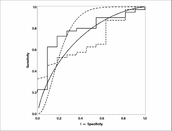
Another sign of poor fit is the unusually large estimates of variability for the model parameters. The estimated values of a and b look normal, but the standard errors are 10 to 20 times larger than model parameters. Although this can happen when estimates are near 0, the estimates in this model are not close to 0.

Be aware that despite their enormous popularity, the binormal models make some strong assumptions. The binormal ROC curve is no longer rank-based; every single observation contributes to the estimation of the binormal slope and intercept. Deviations from normality may have undue influences on the estimated curve and consequences on statistical inference. Generally, there is little reason to use the binormal model to compare ROC curves since methods based on the empirical curve are efficient and implemented in SAS.

You should, however, keep the binormal model in your toolbox. When continuous covariates might affect the predictive accuracy of the marker, empirical ROC methods can no longer be used. You must use model-based techniques, and the binormal model (along with the Lehmann family, covered in subsequent chapters) provides a comprehensive framework from which to draw inferences.

4.7 Bootstrap Confidence Intervals for the Difference in the Area under the Empirical ROC Curve

The bootstrap idea developed in Chapter 3 can be extended to get a confidence interval for the difference in AUCs as well as a p-value for testing whether the difference is significant. The strategy is similar:

• Generate B bootstrap samples.
• For each sample i, compute the AUC of the two ROC curves, AUC₀⁽ⁱ⁾ and AUC₁⁽ⁱ⁾ and compute the difference Δ⁽ⁱ⁾ = AUC₀⁽ⁱ⁾ – AUC₁⁽ⁱ⁾.
• The B numbers, Δ⁽¹⁾ through Δ^(B), approximate the sampling distribution of the difference between the two AUCs.

This can be accomplished by using the %BOOT2AUC macro, which is available from the book's companion Web site at support.sas.com/gonen. The %BOOT2AUC macro is similar to the %BOOT1AUC macro introduced in Section 3.9. The only difference is that it allows for two variable names for the VAR macro variable. For example, the following call requests a comparison of SUV and BSI:

%boot2auc(HeadNeck,suv bsi,ngold);

The results appear in Output 4.3.

Output 4.3

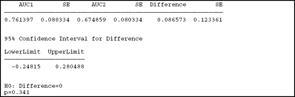
The first part of the output reports the point estimates and standard errors for the individual AUCs as well as their difference. The AUCs and their standard errors are presented and labeled in the order specified in the macro call. The BSI has a bootstrap-estimated AUC of 0.761, and the SUV has 0.675. The difference is 0.087, considerable clinically but not statistically significant with p=0.341 and a confidence interval of (–0.248, 0.280), which includes 0.

4.8 Covariate Adjustment for ROC Curves

In some contexts, covariates influence the accuracy of predictions. In this case, you need to adjust the ROC curve for these covariates. For example, in the context of weather forecasting, the same model that produces the forecasts may have varying accuracy according to the altitude of the geographical location for which the forecasts are produced. In the field of medical diagnosis, certain patient aspects, such as previous exposures to therapy, may influence the ability of diagnostic tools to accurately identify their current medical status. Finally, in the field of credit scoring, the same scoring method may have variable performance in different countries, perhaps due to different legal requirements on how the financial results are reported.

It is important to distinguish a covariate that is a predictor of the outcome as opposed to a covariate that is a risk factor for the outcome. To make this distinction concrete, consider an example from the field of medical diagnostics. Lymphoma is the cancer of lymph nodes. A malignant node is typically enlarged, so the size of a lymph node can be a good predictor of lymphoma. Malignancy, however, is not the only reason that lymph nodes grow. Lymph nodes can be enlarged in patients fighting an infection. Therefore, the size of the lymph node is likely to be a good predictor in patients who did not have a recent infection but a poor predictor if the patient has recently had an infection. On the other hand, whether someone had a recent infection is not a good predictor of lymphoma. Therefore, recent infection is a covariate that may affect the ROC curve but not a covariate that may be used to predict the presence of cancer, neither by itself nor in combination with another predictor.

In contrast, a family history of lymphoma (or perhaps any cancer) makes it more likely for a patient to have cancer because some cancers are genetically inherited. This may be factored into the diagnosis, formally or informally. Whether a patient has a family history of cancer usually has no bearing on whether an enlarged lymph node is a good predictor of cancer. Therefore, a family history of cancer is not a candidate for adjusting ROC curves.

In its simplest form, for a categorical covariate, adjustment implies estimating separate ROC curves for each value of the covariate. With continuous covariates, you can envision an infinite number of ROC curves, one for each possible covariate value. This requires the use of a model that postulates a relationship between the covariate and the parameters of the ROC curves. It should be no surprise that the primary such model is regression. The next section investigates how the binormal model studied in Chapter 3 can be formulated as a regression model.

4.9 Regression Model for the Binormal ROC Curve

The easiest regression model does not contain any covariates. It is not a useful model in practice, but it helps to frame the concepts. In the context of ROC curves, if T denotes the marker and D denotes the disease status (gold standard), then you can write

where ε has a normal distribution with mean 0 and variance σ₀². After some algebra, you can show that

Remember that the coefficient of the variable D represents the difference of the means of the marker for D=1 and D=0. This holds true for any linear model and it will be used in subsequent chapters to extract the information relating to the ROC curve from more complicated models.

This model cannot be fit using the standard linear model procedures in SAS/STAT software, such as GLM or REG. It can be fit, however, with PROC MIXED and, as we saw in Chapter 3, with PROC NLMIXED. PROC MIXED syntax is easier because it follows the general outline of most of the SAS/STAT procedures. On the other hand, PROC NLMIXED can be generalized to the case of ordinal markers as well, as we will see in Chapter 5, so there is a value in adopting PROC NLMIXED as the primary choice of SAS/STAT procedure for modeling ROC curves.

Now we can model the covariates jointly. Consider a binary marker W first:

which implies

These two equations represent the basis for the ROC curves for the two markers implied by the model. Notice that the coefficient of D is the same for both ROC curves. In fact, the two equations differ only in their intercept. Therefore, the implied binormal parameters, a and b, are the same.

You can conclude that adding the covariate as a main effect only does not result in two ROC curves being modeled separately.

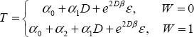
Now consider the following:

which produces the following submodels for W=0 and W=1:

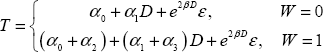
These two submodels generate two different ROC curves since the coefficient of D differs by a factor of α₃.

Specifically for W=0

and for W=1

Note that if α₃=0, the ROC curves for the two markers are identical.

In principle this model can accommodate data collected on two markers. You can create a binary variable for any marker and then use it in place of W to perform the comparison. Typically, there are two practical differences between maker comparison and covariate adjustment:

• Marker comparisons usually involve paired data (as explained in the previous chapter), while covariate adjustments involve unpaired data.
• Marker comparisons usually use a heteroscedastic model (different variances allowed within the two groups defined by the outcome), while covariate adjustments usually employ a homoscedastic model (equal variances assumed within the two groups defined by the outcome).