A.1 Fitting a Simple Linear Model: PROC GLM vs PROC NLMIXED

A.2 PROC NLMIXED and the Binormal Model

PROC NLMIXED plays a central role in this book. Chapters 3, 4, and 5 use it to fit the binormal model, which is one of the fundamental tools to construct and analyze ROC curves.

PROC NLMIXED offers unique and wide-ranging capabilities, but its syntax is different from most other SAS/STAT modeling procedures. For this reason, the PROC NLMIXED code may be difficult to discern and harder to grasp for readers who are used to gaining insight by studying the programs used for model fitting. This appendix is written for users who are familiar with the general SAS/STAT modeling syntax but new to PROC NLMIXED. Regular users of the following procedures may find this appendix helpful: GLM, ANOVA, REG, GENMOD, LOGISTIC, PROBIT, and MIXED.

This appendix is not a summary of all PROC NLMIXED features. Rather, it focuses on capabilities related to ROC curves. SAS/STAT manuals offer exhaustive coverage of PROC NLMIXED and can be helpful for those who want to use this procedure beyond what is covered here.

A.1 Fitting a Simple Linear Model: PROC GLM vs PROC NLMIXED

Consider the following programming statements, which generate a data set of 100 observations. There is a group variable X, taking values of 0 or 1, and an outcome variable Y, which follows a normal distribution within each group. The goal is to fit the following model to this data set using PROC GLM and PROC NLMIXED:

y = α + βX + ε

where ε has a normal distribution with mean 0 and variance σ².

data appendix;
  do i=1 to 100;
    x=rand(‘bernoulli’,0.5);
    e=rannor(0);
    y=x+e;
    output;
  end;
run;

The following statements fit this model in PROC GLM. The MODEL statement in PROC GLM is specifically designed to recognize these special features of this model:

• Presence of an intercept (there is an option for excluding the intercept)
• Linearity of the model term
• Normal distribution of the error terms with constant variance.

For these reasons, it is sufficient to write model y=x.

title “Simple Linear Model Using GLM”;
proc glm;
   model y=x;
run;
quit;

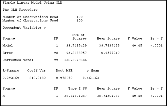
Output A.1 shows the results from PROC GLM. The parameter estimates for α (labeled Intercept) and β (labeled X) are −0.241 and 1.254, with standard errors of 0.148 and 0.197. An estimate of σ² is provided by the mean squared error (0.9578).

Output A.1

PROC NLMIXED does not have a MODEL statement with these features. Rather, the model needs to be communicated to PROC NLMIXED step by step, with specific instructions on the model and the distribution of the variables. The following PROC NLMIXED code fits the same model:

title “Simple Linear Model Using NLMIXED”;
proc nlmixed;
   parms var=1 alpha=0 beta=0;
   mu=alpha+x*beta;
   model y~normal(mu,var);
run;
quit;

It is most useful to deconstruct PROC NLMIXED programs starting from the end. The MODEL statement has no resemblance to the one in PROC GLM. The equal sign is replaced by the tilde (~), which is read as “distributed as.” Hence, this model statement is specifying that the response variable Y has a normal distribution with mean MU and standard deviation VAR. A key difference between PROC GLM syntax and PROC NLMIXED syntax is that in PROC NLMIXED, only parameters are allowed on the right-hand side of a MODEL statement, whereas in PROC GLM, only variables are allowed.

The statement mu=alpha+x*beta connects the model parameters to the data set variables. It specifies that the mean of the normal distribution is related to the covariate X in a linear fashion. Most DATA step functions are available for programming in PROC NLMIXED, so you can construct almost any functional relationship between parameters.

Finally, the PARMS statement tells PROC NLMIXED which of the terms are parameters. The PARMS statement is not required. In its absence, PROC NLMIXED assumes that any term that is not assigned a value, either from the data set or from the programming statements within the procedure, is a parameter. In this case, it is easy to check that omitting the PARMS statement does not alter the output. In more complicated models, the PARMS statement helps you keep track of the model parameters. The numbers following the equal sign after the parameter names are the starting values for the numerical search method employed by PROC NLMIXED. They can be safely ignored for the time being until we briefly discuss the implications of using the maximum likelihood in PROC NLMIXED later in this appendix.

The output from this invocation of PROC NLMIXED appears here. The parameter estimates for α, β, and σ² are −0.241, 1.254, and 0.9386, with standard errors 0.148, 0.197, and 0.1327. The estimates for α and β are identical to the ones provided by PROC GLM (up to rounding), but the estimates for σ² seem to differ slightly (0.9578 vs. 0.9386). This discrepancy results from the different estimation methods used by the two procedures. It is usually small, especially with moderate to large sample sizes. We will discuss this next.

Output A.2

PROC GLM uses the method of least squares to find the estimates. Least squares equations for a given statistical linear model have closed form solutions; that is, you can solve a set of linear equations to obtain the estimates. The information in the PROC GLM output such as the sum of squares and mean squares are all related to the analysis of variance decomposition of the total sum of squares, a concept closely connected to the least squares methodology.

In contrast, PROC NLMIXED uses likelihood-based methods. These methods are very general. They can be used effectively for nonlinear or nonnormal models. The price of the generality is the lack of closed-form solutions. In general, likelihood equations are nonlinear and can only be solved by numerical search algorithms. For example, under the Specifications heading in the PROC NLMIXED output, the method of optimization is listed as Dual Quasi-Newton. This is one method of solving the likelihood equations to obtain the estimates. The Dual Quasi-Newton algorithm (and others used in PROC NLMIXED, which can be specified by the METHOD option in the procedure statement) is iterative. The algorithm takes small steps, called iterations, toward the solution. The starting point of the iterations are the ones listed (after the equal signs) in the PARAMS statement. The listing under Iteration History in the output gives details of each such iteration. This table is normally useful only to advanced users of PROC NLMIXED.

The reason for the slight difference in the estimates of σ² is that the maximum likelihood estimates use n (total sample size) as the denominator for the variance estimates, whereas the least squares methods use n–p, where p is the number of model parameters. To the extent that p is small compared to n, the estimates will be close. You can obtain the maximum likelihood estimate from the PROC GLM output by dividing the error sum of squares (93.8639) by 100.

Model fit is assessed by likelihood-based criteria such as Akaike's Information Criterion (AIC) or Bayes Information Criterion (BIC) in PROC NLMIXED, which are reported under Fit Statistics. These are useful for model comparison. Users of PROC MIXED, another procedure that used likelihood methods, will be familiar with these criteria. In contrast, model fit in PROC GLM is usually assessed by the omnibus F-test, which is a function of the sum of squares.

The structure of the Parameter Estimates table is similar to the output of other SAS/STAT programs. There is normally another column labeled Alpha in the output, reporting the significance level used in the confidence intervals, which is removed here to save space. An additional piece of information, the value of the gradient at the final iteration, is also provided but is likely to benefit only advanced users.

A.2 PROC NLMIXED and the Binormal Model

It may be useful to understand how the PROC NLMIXED programs used in Chapters 3 and 5 are developed. First, consider the model and code from Section 3.5:

proc nlmixed;
  parms m1=0 m0=0 s1=1 s0=1;
  if gold=1 then m=m1;else if gold=0 then m=m0;
  if gold=0 then s=s1**2;else if gold=0 then s=s0**2;
  a=(m1-m0)/s1;
  b=s0/s1;
  model y~normal(m,s);
  estimate ‘a’ a;
  estimate ‘b’ b;
  estimate ‘AUC’ probnorm(a/sqrt(1+b**2)));
run;
quit;

The MODEL statement specifies a normally distributed outcome with mean M and variance S, which are defined by the two IF statements. This would produce an ROC analysis, but you would have to manually (or in a DATA step) generate point estimates for the binormal parameters a and b, as well as the area under the ROC curve (AUC). Obtaining their variances would take considerable time and some knowledge of PROC IML. This underscores the practicality of the ESTIMATE statement, where you can define any nonlinear transformation using a DATA step-like programming approach and obtain the point estimates and standard errors. The following code shows two different ways of doing so:

1. These quantities can be defined first and then estimated. This method was used for the binormal parameters a and b in the code above.
2. The definition can be performed in the ESTIMATE step. This method was used for the AUC in the code above.

Note that the ESTIMATE statement in PROC GLM and other SAS/STAT procedures works only with linear transformation, so obtaining estimates of a, b, and AUC is not possible with, say, PROC GLM.

Now let's revisit the latent binormal model from Chapter 5. This highlights a major strength of PROC NLMIXED: the ability to specify an arbitrary likelihood function.

proc nlmixed data=moody gconv=0;
   parms alpha=1 theta1=1 theta2=2 theta3=3 beta=1;
   bounds theta1>0, theta2>0, theta3>0;
   eta1=alpha*def;
   eta2=exp(beta*def);
        if r11=1 then z=probnorm(-eta1/eta2);
   else if r11=2 then z=probnorm((theta1-eta1)/eta2)-
       probnorm(-eta1/eta2);
   else if r11=3 then z=probnorm((theta2+theta1-eta1)/eta2)-
       probnorm((theta1-eta1)/eta2);
   else if r11=4 then z=probnorm((theta3+theta2+theta1-eta1)/eta2)-
       probnorm((theta2+theta1-eta1)/eta2);
   else if r11=5 then z=1 - probnorm((theta3+theta2+theta1-
      eta1)/eta2);
   if z>1e-6 then ll=log(z);
      else ll=-1e6;
   model r11 ~ general(ll);
   estimate ‘AUC’ probnorm(alpha/sqrt(1+beta**2));
run;

The MODEL statement specifies a GENERAL (LL) model. This means that the (logarithm of the) likelihood function is being defined by the user through term LL. Recall that R11 represents the ordinal credit scores and the underlying model is a latent ordinal regression model. Each IF statement specifies the contribution to the likelihood from every possible value of R11, the ordinal ratings. These contributions were derived in Chapter 5 to be

The structure of the IF statements mimics this formulation closely. These statements uniquely define a value for Z, the likelihood, and hence LL, which is the logarithm of Z. The condition that the contributions to the likelihood that are less than 10^-6 will be counted as 10^-6 ensures that very small contributions do not cause numerical instability.