Chapter 3
Preliminary and Background Information
Contents
3.1 What Every Programmer Should Know before Simulating Data
3.2 Essential Functions for Working with Statistical Distributions
3.2.1 The Probability Density Function (PDF)
3.2.2 The Cumulative Distribution Function (CDF)
3.2.3 The Inverse CDF (QUANTILE Function)
3.2.4 The Older SAS Random Number Functions
3.3 Random Number Streams in SAS
3.3.1 Setting a Seed Value for Random Number Generation
3.3.2 Setting a Seed Value from the System Time
3.4 Checking the Correctness of Simulated Data
3.4.1 Sample Moments and Goodness-of-Fit Tests
3.4.2 Overlay a Theoretical PMF on a Frequency Plot
3.4.3 Overlaying a Theoretical Density on a Histogram
3.4.4 The Quantile-Quantile Plot
3.5 Using ODS Statements to Control Output
3.5.1 Finding the Names of ODS Tables
3.5.2 Selecting and Excluding ODS Tables
3.5.3 Creating Data Sets from ODS Tables
3.1 What Every Programmer Should Know before Simulating Data
This chapter describes basic statistical distributional theory and details of SAS software that are essential to know before you begin simulating data. This chapter lays the foundation for how to efficiently simulate data in SAS software. In particular, this chapter describes the following:
- How to use four essential functions for working with statistical distributions. In SAS software, these functions are the PDF, CDF, QUANTILE, and RAND (or RANDGEN) functions.
- How to control random number streams in SAS software.
- How to check the correctness of simulated data.
- How to control output from SAS procedures by using the Output Delivery System (ODS).
If you are already familiar with these topics, then you can skip this chapter.
3.2 Essential Functions for Working with Statistical Distributions
If you work with statistical simulation, then it is essential to know how to compute densities, cumulative densities, quantiles, and random values for statistical distributions. In SAS software, the four functions are computed by using the PDF, CDF, QUANTILE, and RAND (or RANDGEN) functions.
- The PDF function evaluates the probability density function for continuous distributions and the probability mass function (PMF) for discrete distributions. For continuous distributions, the PDF function returns the probability density at the specified value. For discrete distributions, it returns the probability that a random variable takes on the specified value.
- The CDF function computes the cumulative distribution function. The CDF returns the probability that an observation from the specified distribution is less than or equal to a particular value. For continuous distributions, this is the area under the density curve up to a certain point.
- The QUANTILE function is closely related to the CDF function, but solves an inverse problem. Given a probability, P, the quantile for P is the smallest value, q, for which CDF(q) is greater than or equal to P.
- The RAND function generates a random sample from a distribution. In SAS/IML software, use the RANDGEN subroutine, which fills up an entire matrix with random values. Examples of using these functions are given in Chapter 2, “Simulating Data from Common Univariate Distributions,” and throughout this book.
3.2.1 The Probability Density Function (PDF)
The probability density function is often used to define a distribution. For example, the PDF for the standard normal distribution is ɸ(x) = (1/![]() )exp(–x2/2). You can use the PDF function to draw the graph of the probability density function. For example, the following SAS program uses the DATA step to generate points on the graph of the standard normal density, as follows:
)exp(–x2/2). You can use the PDF function to draw the graph of the probability density function. For example, the following SAS program uses the DATA step to generate points on the graph of the standard normal density, as follows:
data pdf;
do x = -3 to 3 by 0.1;
   y = pdf(“Normal”, x);
   output;
end;
run;
Figure 3.1 Standard Normal Probability Density

Figure 3.1 shows the graph of the standard normal PDF and the evaluation of the PDF at the points x = 0 and x = 1. The graph shows that ɸ(0) is a little less than 0.4 and that ɸ(1) is close to 0.25. This book's Web site provides SAS code that generates this and all other figures in this book.
Exercise 3.1: Use the SGPLOT procedure to plot the PDF of the standard exponential distribution.
3.2.2 The Cumulative Distribution Function (CDF)
The cumulative distribution function returns the probability that a value drawn from a given distribution is less than or equal to a given value.
For a continuous distribution, the CDF is the integral of the PDF from the lower range of the distribution (often –∞) to the given value. For example, for the standard normal distribution, the CDF at x = 0 is 0.5 because that is the area under the normal curve to the left of 0. For a discrete distribution, the CDF is the sum of the PMF for all values less than or equal to the given value.
The CDF of any distribution is a non-decreasing function. For the familiar continuous distributions, the CDF is monotone increasing. For discrete distributions, the CDF is a step function. The following DATA step generates points on the graph of the standard normal CDF. Figure 3.2 shows the graph of the CDF for the standard normal distribution and the evaluation of the CDF at x = 0 and x = 1.645. The graph shows that CDF(0) = 0.5 and CDF(1.645) = 0.95.
data cdf;
do x = -3 to 3 by 0.1;
   y = cdf(“Normal”, x);
   output;
end;
run;
Figure 3.2 Standard Normal Cumulative Density

Exercise 3.2: Use the SGPLOT procedure to plot the CDF of the standard exponential distribution.
3.2.3 The Inverse CDF (QUANTILE Function)
If the CDF is continuous and strictly increasing, then there is a unique answer to the question: Given an area (probability), what is the value q for which the integral up to q has the specified area? The value q is called the quantile for the specified probability distribution. The median is the quantile of 0.5, the 90th percentile is the quantile of 0.9, and so on. For discrete distributions, the quantile is the smallest value for which the CDF is greater than or equal to the given probability.
For the standard normal distribution, the quantile of 0.5 is 0, and the 95th percentile is 1.645. You can find a quantile graphically by using the CDF plot: Choose a value q between 0 and 1 on the vertical axis, and use the CDF curve to find the value of x whose CDF is q, as shown in Figure 3.2.
Quantiles are used to compute p-values for hypothesis testing. For symmetric distributions, such as the normal distribution, the quantile for 1 − α/2 is used to compute two-sided p-values. For example, when α = 0.05, the (1 − α/2) quantile for the standard normal distribution is computed by quantile(“Normal”, 0.975), which is the famous number 1.96.
3.2.4 The Older SAS Random Number Functions
Long-time SAS users might remember the older PROBXXX, XXXINV, and RANXXX functions for computing the CDF, inverse CDF (quantiles), and for sampling. For example, you can use the PROBGAM, GAMINV, and RANGAM functions for working with the gamma distribution. (For the normal distribution, the older names are PROBNORM, PROBIT, and RANNOR.) Although SAS still supports these older functions, you should not use them for simulations that generate many millions of random values. These functions use an older random number generator whose statistical properties are not as good as those of the newer Mersenne-Twister random number generator (Matsumoto and Nishimura 1998), which is known to have excellent statistical properties.
One of the desirable properties of the Mersenne-Twister algorithm is its extremely long period. The period of a random number stream is the number of uniform random numbers that you can generate before the sequence begins to repeat. The older RANXXX functions have a period of about 231, which is about 2 × 10⁹, whereas the Mersenne-Twister algorithm has a period of about 219937, which is about 4 × 106001. For comparison, the number of atoms in the observable universe is approximately 1080.
3.3 Random Number Streams in SAS
Often the term “random number” means a number sampled from the uniform distribution on [0, 1]. Random values for other distributions are generated by transformations of one or more uniform random variates. The seed value that controls the generation of uniform random variates also controls the generation of random variates for any distribution.
You can generate random numbers in SAS by using the RAND function in the DATA step or by using the RANDGEN subroutine in SAS/IML software. The functions call the same underlying numerical algorithms. These functions generate a stream of random variates from a specified distribution. You can control the stream by setting the seed for the random numbers. For the RAND function, the seed value is set by using the STREAMINIT subroutine; for the RANDGEN subroutine, use the RANDSEED subroutine in the SAS/IML language.
Specifying a particular seed enables you to generate the same set of random numbers every time that you run the program. This seems like an oxymoron: If the numbers are the same every time, then how can they be random? The resolution to this paradox is that the numbers that we call “random” should more accurately be called “pseudorandom” numbers. Pseudorandom numbers are generated by an algorithm, but have statistical properties of randomness. A good algorithm generates pseudorandom numbers that are indistinguishable from truly random numbers.
Why would you want a reproducible sequence of random numbers? Documentation and testing are two important reasons. Each example in this book explicitly sets a seed value (such as 4321) so that you can run the programs and obtain the same results.
3.3.1 Setting a Seed Value for Random Number Generation
The STREAMINIT subroutine is used to set the seed value for the RAND function in the DATA step. The seed value controls the sequence of random numbers. Syntactically, you should call the STREAMINIT subroutine one time per DATA step, prior to the first invocation of the RAND function. It does not make sense to call STREAMINIT multiple times within the same DATA step; subsequent calls are ignored.
A DATA step or SAS procedure produces the same pseudorandom numbers when given the same seed value. This means that you need to be careful when you write a single program that contains multiple DATA steps that each generate random numbers. In this case, use a different seed value in each DATA step or else the streams will not be independent. For example, the following DATA steps generate exactly the same simulated data:
data a;
call streaminit(4321);
do i = 1 to 10; x=rand(“uniform”); output; end;
run;

data b;
call streaminit(4321);
do i = 1 to 10; x=rand(“uniform”); output; end;
run;

proc compare base=a compare=b; run;      /* show they are identical */
This advice also applies to writing a macro function that generates random numbers. Do not explicitly set a seed value inside the macro. If you do, then each run of the macro will generate the same values. Rather, enable the user to specify the seed value in the syntax of the macro.
3.3.2 Setting a Seed Value from the System Time
If you do not explicitly call STREAMINIT, then the first call to the RAND function implicitly calls STREAMINIT with 0 as an argument. If you use a seed value of 0, then the STREAMINIT function uses the time on the internal system clock as the seed value. In this case, the random number stream is different each time you run the program.
However, “different each time” does not mean that the random number stream is not reproducible. SAS provides a macro variable named SYSRANDOM that contains the most recent seed value. If you explicitly set the seed value (for example, 4321), then the SYSRANDOM macro variable contains that value. If you specify a value of zero, then the system clock is used to generate a value such as 488637001. After the DATA step exits, the SYSRANDOM macro variable is set to that value. You can use the value as a seed to reproduce the same stream. For example, in the following program the first DATA step generates a random number stream by using the system clock. The SYSRANDOM macro is used in the second DATA step, which results in an identical set of random values, as shown in Figure 3.3.
data a;
call streaminit(0);                    /* different stream each time */
do i = 1 to 10; x=rand(“uniform”); output; end;
run;

data b;
call streaminit(&sysrandom);     /* use SYSRANDOM to set same seed */
do i = 1 to 10; x=rand(“uniform”); output; end;
run;

proc compare base=a compare=b short;     /* show they are identical */
run;
Figure 3.3 Identical Random Number Streams

To show the seed value that was used, use the %PUT statement to display the value of the SYSRANDOM macro variable in the SAS log.
3.4 Checking the Correctness of Simulated Data
Whenever you implement an algorithm, it is a good idea to test whether your implementation is correct. Although it is usually quite difficult (or impossible) to rigorously test that simulated data are truly a sample from a specified distribution, there are four quick ways to check that you have not made a major error. Generate a large sample, and do one or more of the following:
- Compare sample moments of the simulated data with theoretical moments of the underlying distribution.
- Compare the empirical CDF with the theoretical cumulative distribution by using statistical goodness-of-fit tests.
- Compare the frequency or density of the simulated data with the theoretical PMF or PDF. To do this, create a bar chart or histogram of the simulated data and overlay the PMF or PDF, respectively, of the distribution.
- Compare empirical quantiles of the simulated data with theoretical quantiles. For continuous distributions, construct a quantile-quantile plot that compares quantiles of the simulated data to theoretical quantiles of the distribution. This is shown in Section 3.4.4. For discrete distributions, there are plots that serve a similar purpose (Friendly 2000).
3.4.1 Sample Moments and Goodness-of-Fit Tests
The UNIVARIATE procedure can be used to carry out these four checks for a variety of commonly used continuous distributions.
For example, the gamma distribution with shape parameter α and scale parameter σ is denoted by Gamma(α, σ). Its density is
![]()
where Г(α) is the gamma function. When a is an integer, Г(α) = (α − 1)!. When σ = 1, the gamma distribution is denoted Gamma(α).
The following statements simulate observations from a gamma distribution with shape parameter α = 4 and unit scale. PROC UNIVARIATE is then called to compute the sample moments (see Figure 3.4) and to perform a goodness-of-fit test (see Figure 3.5).
%let N=500;
data Gamma(keep=x);
call streaminit(4321);
do i = 1 to &N;
   x = rand(“Gamma”, 4);         /* shape=4, unit scale */
   output;
end;
run;

/* fit Gamma distrib to data; compute GOF tests */
proc univariate data=Gamma;
   var x;
   histogram x / gamma(alpha=EST scale=1);
   ods select Moments ParameterEstimates GoodnessOfFit;
run;
Figure 3.4 Sample Moments

For a gamma distribution with unit scale and shape parameter α, the mean and variance are α, the skewness is 2/![]() , and the (excess) kurtosis is 6/α. When α = 4, these values are 4, 4, 1, and 1.5. Figure 3.4 shows the sample moments for the simulated data, which are 4.04, 4.21, 0.98, and 0.91. The standard errors of the mean and variance are smaller than for the skewness and kurtosis, so you should expect the mean and variance to be closer to the corresponding population parameters than the skewness and kurtosis are.
, and the (excess) kurtosis is 6/α. When α = 4, these values are 4, 4, 1, and 1.5. Figure 3.4 shows the sample moments for the simulated data, which are 4.04, 4.21, 0.98, and 0.91. The standard errors of the mean and variance are smaller than for the skewness and kurtosis, so you should expect the mean and variance to be closer to the corresponding population parameters than the skewness and kurtosis are.
Figure 3.5 shows the results of fitting a Gamma(α) distribution (with unit scale) to the simulated data. The maximum likelihood estimate of α is α = 4.03. The goodness-of-fit tests all have large p-values, which indicates that there is no reason to doubt that the data are a random sample from a gamma distribution. However, as discussed in the documentation for the UNIVARIATE procedure in the Base SAS Procedures Guide: Statistical Procedures, “A test's ability to reject the null hypothesis (known as the power of the test) increases with the sample size.” In practical terms, this means that for a large sample the goodness-of-fit tests often have small p-values, even if the sample is drawn from the fitted distribution.
Figure 3.5 Goodness-of-Fit Tests

Exercise 3.3: Simulate N =10,000 observations from the Gamma(4) distribution and compute the sample moments. Are the estimates closer to the parameter values than for the smaller sample size? What are the p-values for the goodness-of-fit tests?
3.4.2 Overlay a Theoretical PMF on a Frequency Plot
When you implement a sampling algorithm, it is good programming practice to check the validity of the algorithm. Overlaying the theoretical probabilities is one way to check whether the sample appears to be from the specified distribution. You can use the Graph Template Language (GTL) to define a template for a scatter plot overlaid on a bar chart. The bar chart displays the empirical frequencies of a sample whereas the scatter plot shows the probability mass function (PMF) for the population.
For example, suppose that you want to draw a random sample from the geometric distribution and overlay the PMF on the empirical frequencies. There are two common definitions for a geometric random variable. Let B1, B2,…be a sequence of independent Bernoulli trials with probability p. Then either of the following definitions are used for a geometric random variable with parameter p:
- the number of trials until the first success
- the number of trials up to but not including the first success
The two definitions are interchangeable because if X is a geometric random variable that satisfies the first definition, then X − 1 is a random variable that satisfies the second definition. SAS uses both definitions. The first definition is used by the RAND and RANDGEN functions, whereas (regrettably) the PDF function uses the second definition. Notice that a random variable that obeys the first definition takes on positive values; for the second definition, the variable is nonnegative.
The following DATA step draws 100 observations from the geometric distribution with parameter 0.5. Intuitively, this is a simulation of 100 experiments in which a coin is tossed until heads appears, and the number of tosses is recorded.
%let N=100;
data Geometric(keep=x);
call streaminit(4321);
do i = 1 to &N;
   x = rand(“Geometric”, 0.5);         /* number of tosses until heads */
   output;
end;
run;
The distribution of the simulated data can be compared with the PMF for the geometric distribution, which is computed by using the following DATA step:
/* For the geometric distribution, PDF(“Geometric”, t, 0.5) computes the
   probability of t FAILURES, t=0, 1, 2,… Use PDF(“Geometric”, t-1, 0.5)
   to compute the number of TOSSES until heads appears, t=1, 2, 3,…. */
data PMF(keep=T Y);
do T = 1 to 9;
   Y = pdf(“Geometric”, T-1, 0.5);
   output;
end;
run;
The x variable in the Geometric data set contains 100 observations. The PMF data set contains nine observations. Nevertheless, you can merge these two data sets to create a single data set that contains all the data to be plotted:
data Discrete;
   merge Geometric PMF;
run;
The SGPLOT procedure does not support overlaying a bar chart and a scatter plot, so you need to use the GTL and PROC TEMPLATE to create a template that defines the layout of the graph. The template consists of three overlays: a bar chart, a scatter plot, and (optionally) a legend. The following statements define the template and render the graph by calling the SGRENDER procedure. Figure 3.6 shows the resulting graph. A short macro is used to handle the fact that the STAT= option in the BARCHART statement changed between SAS 9.3 and SAS 9.4.
/* GTL syntax changed at 9.4 */
%macro ScaleOpt;
   %if %sysevalf(&SysVer < 9.4) %then pct; %else proportion;
%mend;
proc template;
define statgraph BarPMF;
dynamic _Title;            /* specify title at run time */
begingraph;
   entrytitle _Title;
   layout overlay / yaxisopts=(griddisplay=on)
                    xaxisopts=(type=discrete);
   barchart x=X / name=‘bar’ legendlabel=‘Sample’ stat=%ScaleOpt;
   scatterplot x=T y=Y / name=‘pmf’ legendlabel=‘PMF’;
   discretelegend ‘bar’ ‘pmf’;
   endlayout;
endgraph;
end;
run;

proc sgrender data=Discrete template=BarPMF;
   dynamic _Title = “Sample from Geometric(0.5) Distribution (N=&N)”;
run;
Figure 3.6 Sample from Geometric Distribution (p = 0.5) Overlaid with PMF

The BarPMF template is a simplified version of the template that is used for this book. (You can download the full version from the book's Web site.) Notice that the template uses a DYNAMIC statement to set the title of the graph. The title is set when the SGRENDER procedure is called. Although this is not necessary, it is convenient because you can reuse the template for many data sets. You can also use the DYNAMIC statement to specify other parts of the graph (for example, the names of the X, T, and Y variables) at run time.
Exercise 3.4: A negative binomial variable is defined as the number of failures before k successes in a series of independent Bernoulli trials with probability of success p. Sample 100 observations from a negative binomial distribution with p = 0.5 and k = 3 and overlay the PMF.
3.4.3 Overlaying a Theoretical Density on a Histogram
This section uses the Graph Template Language (GTL) to define a template for a density curve (PDF) overlaid on a histogram. For many distributions, you can use the HISTOGRAM statement in PROC UNIVARIATE to overlay a PDF on a histogram. However, using the GTL enables you to overlay density curves for families that are not supported by PROC UNIVARIATE.
As an example, suppose that you want to draw a random sample from the gamma distribution and overlay the PDF on the empirical distribution. Section 3.4.1 created the Gamma data set, which contains 500 observations from the Gamma(4) distribution. The PDF for the gamma distribution is computed by using the following DATA step:
data PDF(keep=T Y);
do T = 0 to 13 by 0.1;
   Y = pdf(“Gamma”, T, 4);
   output;
end;
run;
The Gamma data set contains 500 observations. The PDF data set contains fewer observations. You can merge these two data sets to create a single data set that contains all the data to be plotted:
data Cont;
   merge Gamma PDF;
run;
The SGPLOT procedure in SAS 9.3 does not support overlaying a histogram and a custom density curve, so you need to use the GTL and PROC TEMPLATE to create a template that defines the layout of the graph. The template consists of three overlays: a histogram, a series plot, and (optionally) a legend. The following statements define the template and render the graph by calling the SGRENDER procedure. Figure 3.7 shows the resulting graph.
proc template;
define statgraph HistPDF;
dynamic _Title _binstart _binstop _binwidth;
begingraph;
   entrytitle _Title;
   layout overlay / xaxisopts=(linearopts=(viewmax=_binstop));
   histogram X / scale=density endlabels=true xvalues=leftpoints
         binstart=_binstart binwidth=_binwidth;
   seriesplot x=T y=Y / name=‘PDF’ legendlabel=“PDF”
         lineattrs=(thickness=2);
   discretelegend ‘PDF’;
   endlayout;
endgraph;
end;
run;

proc sgrender data=Cont template=HistPDF;
dynamic _Title=“Sample from Gamma(4) Distribution (N=&N)”
   _binstart=0            /* left endpoint of first bin */
   _binstop=13            /* right endpoint of last bin */
   _binwidth=1;           /* width of bins              */
run;
Figure 3.7 Sample from Gamma(4) Distribution Overlaid with PDF

The HistPDF template is a simplified version of the template used for this book. (You can download the full version from the book's Web site.) Notice that the template uses a DYNAMIC statement to set the title of the graph and also to set three parameters that are used to specify the histogram bins. These parameters are set when the SGRENDER procedure is called. Specifying these parameters at run time enables you to use the template for many data sets. You can also define the names of the three variables as dynamic variables.
Exercise 3.5: Simulate 500 observations from a chi-square distribution with 3 degrees of freedom and overlay the PDF.
3.4.4 The Quantile-Quantile Plot
When you generate a sample from a continuous univariate distribution, you can use a quantile-quantile plot (Q-Q plot) to plot the ordered values of the sample against quantiles of the assumed distribution (Chambers et al. 1983). If the data are a sample from the specified distribution, then the points on the plot tend to fall along a straight line.
There are two ways to create a Q-Q plot in SAS. For many standard distributions, you can use the QQPLOT statement in PROC UNIVARIATE. In the following example, an exponential model is fit to simulated data. The Q-Q plot is shown in Figure 3.8.
data Exponential(keep=x);
call streaminit(4321);
sigma = 10;
do i = 1 to &N;
   x = sigma * rand(“Exponential”);
   output;
end;
run;

/* create an exponential Q-Q plot*/
proc univariate data=Exponential;
   var x;
   qqplot x / exp;
run;
Figure 3.8 Exponential Q-Q Plot

The points in the exponential Q-Q plot fall along a straight line. Therefore, there is no reason to doubt that the data are a random sample from an exponential distribution. The slope of the line is an estimate of the exponential scale parameter, which is 10 for this example. For more information about the interpretation of Q-Q plots, see “Interpretation of Quantile-Quantile and Probability Plots” in the PROC UNIVARIATE documentation in the Base SAS Procedures Guide: Statistical Procedures.
A second way to create a Q-Q plot is to manually compute the quantiles and use the SGPLOT procedure to create the graph. The advantage of this approach is that you can handle any distribution for which you can compute the inverse CDF. This approach requires the following steps:
- Sort the data.
- Compute n evenly spaced points in the interval (0, 1), where n is the number of data points in the sample.
- Compute the quantiles (inverse CDF) of the evenly spaced points.
- Create a scatter plot of the sorted data versus the quantiles.
The steps are implemented by the following statements, which create a normal Q-Q plot. The Q-Q plot is shown in Figure 3.9.
%let N = 100;
data Normal(keep=x);
call streaminit(4321);
do i = 1 to &N;
   x = rand(“Normal”);                         /* N(0, 1) */
   output;
end;
run;

/* Manually create a Q-Q plot */
proc sort data=Normal out=QQ; by x; run;             /* 1 */

data QQ;
set QQ nobs=NObs;
v = (_N_ - 0.375) / (NObs + 0.25);                   /* 2 */
q = quantile(“Normal”, v);                           /* 3 */
label x = “Observed Data” q = “Normal Quantiles”;
run;

proc sgplot data=QQ;                                 /* 4 */
   scatter x=q y=x;
   xaxis grid; yaxis grid;
run;
Figure 3.9 Normal Q-Q Plot

The points in the normal Q-Q plot fall along a straight line. Therefore, there is no reason to doubt that the simulated data are normally distributed. Furthermore, because the data in the Q-Q plot appear to pass through the origin and have unit slope, the parameter estimates for the normal fit to the data are close to μ = 0 and σ = 1.
The previous technique enables you to compute a Q-Q plot for any continuous distribution. Simply replace the “Normal” parameter in the QUANTILE function with “Exponential” or “Lognormal” to obtain a Q-Q plot for those distributions.
Exercise 3.6: Simulate data from the N(1, 3) distribution. Create a normal Q-Q plot of the data. Do the points of the plot appear to fall along a line that has 1 as a y -intercept and 3 for a slope?
Exercise 3.7: Section 3.4 creates a Gamma data set that contains a random sample from the Gamma(4) distribution. Manually create a Q-Q plot, and verify that it is the same as is produced by the QQPLOT statement in PROC UNIVARIATE.
3.5 Using ODS Statements to Control Output
The SAS Output Delivery System (ODS) enables you to control the output from SAS programs. SAS procedures use ODS to display results. Most results are displayed as ODS tables; ODS statistical graphics are discussed briefly in Section 3.5.4.
There are ODS statements that enable you to control the output that is displayed, the destination for the output (such as the LISTING or HTML destinations), and many other aspects of the output. This section describes a few elementary ODS statements that are used in this book. For a more complete description, see the SAS Output Delivery System: User's Guide.
3.5.1 Finding the Names of ODS Tables
Before you can include, exclude, or save tables, you need to know the names of the tables. You can determine the names of ODS tables by using the ODS TRACE statement. The most basic syntax is as follows:
ODS TRACE ON | OFF ;
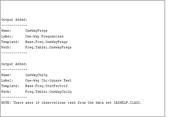
When you turn on tracing, SAS software displays the names of subsequent ODS tables that are produced. The names are usually printed to the SAS log. For example, the following statements display the names of tables that are created by the FREQ procedure during a frequency analysis of the Sex variable in the Sashelp.Class data set:
ods trace on;
ods graphics off;
proc freq data=Sashelp.Class;
   tables sex / chisq;
run;
ods trace off;
The content of the SAS log is shown in Figure 3.10. The FREQ procedure creates two tables: the OneWayFreqs table and the OneWayChiSq table.
Figure 3.10 Names of ODS Tables
3.5.2 Selecting and Excluding ODS Tables
You can limit the output from a SAS procedure by using the ODS SELECT and ODS EXCLUDE statements. The ODS SELECT statement specifies the tables that you want to display; the ODS EXCLUDE statement specifies the tables that you want to suppress. The basic syntax is as follows:
ODS SELECT table-names | ALL | NONE ;
ODS EXCLUDE table-names | ALL | NONE ;
For example, PROC FREQ will display only the OneWayChiSq table if you specify either of the following statements:
ods select OneWayChiSq;
ods exclude OneWayFreqs;
3.5.3 Creating Data Sets from ODS Tables
You can use the ODS OUTPUT statement to create a SAS data set from an ODS table. For example, use the following statements to create a SAS data set named Freqs from the OneWayFreqs table that is produced by PROC FREQ:
proc freq data=Sashelp.Class;
   tables sex;
   ods output OneWayFreqs=Freqs;
run;
You can then use the data set as input for another procedure. This technique is especially useful when you need to save a statistic that appears in a table, but the procedure does not provide an option that writes the statistic to an output data set.
Of course, you typically need to know the names of the variables in the data set before you can use the data. You can use PROC CONTENTS to display the variable names as shown in the following statements:
proc contents data=Freqs short order=varnum;
run;
Figure 3.11 Variable Names

3.5.4 Creating ODS Statistical Graphics
Many SAS procedures support ODS statistical graphics. You can use the ODS GRAPHICS statement to initialize the ODS statistical graphics system. The basic syntax is as follows:
ODS GRAPHICS ON | OFF ;
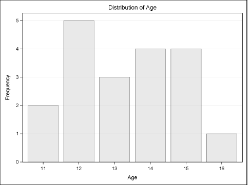
You can use the ODS SELECT and ODS EXCLUDE statements on graphical objects just as you can for tabular output. For example, the following statements perform a frequency analysis on the Age variable in the Sashelp.Class data set. The ODS SELECT statement excludes all output except for the bar chart that is shown in Figure 3.12.
ods graphics on;
proc freq data=Sashelp.Class;
   tables age / plot=FreqPlot;
   ods select FreqPlot;
run;
Figure 3.12 An ODS Graphic
3.6 References
Chambers, J. M., Cleveland, W. S., Kleiner, B., and Tukey, P. A. (1983), Graphical Methods for Data Analysis, Belmont, CA: Wadsworth International Group.
Friendly, M. (2000), Visualizing Categorical Data, Cary, NC: SAS Institute Inc.
Matsumoto, M. and Nishimura, T. (1998), “Mersenne Twister: A 623-Dimensionally Equidistributed Uniform Pseudo-random Number Generator,” ACM Transactions on Modeling and Computer Simulation, 8, 3–30.