Appendix A
A SAS/IML Primer
Contents
A.1 Overview of the SAS/IML Language
A.2 SAS/IML Functions That Are Used in This Book
A.4 Subscript Reduction Operators in SAS/IML Software
A.5 Reading Data from SAS Data Sets
A.5.1 Reading Data into SAS/IML Vectors
A.5.2 Creating Matrices from SAS Data Sets
A.6 Writing Data to SAS Data Sets
A.6.1 Creating SAS Data Sets from Vectors
A.6.2 Creating SAS Data Sets from Matrices
A.9 Modules That Replicate SAS/IML Functions
A.1 Overview of the SAS/IML Language
The SAS/IML language is a high-level matrix language that enables SAS users to develop algorithms and compute statistics that are not built into any SAS procedure. The language contains hundreds of built-in functions for statistics, data analysis, and matrix computations, and enables you to call hundreds of DATA step functions. You can write your own functions to extend the language.
If you are serious about simulating data (especially multivariate data), you should take the time to learn the SAS/IML language. The following resources can help you get started:
- Read chapters 1-4 and 13-15 of Statistical Programming with SAS/IML Software (Wicklin 2010).
- Subscribe to The DO Loop blog, which is a statistical programming blog that is located at the URL
blogs.sas.com/content/iml. - Ask questions at the SAS/IML Community, which is located at
communities.sas.com/community/support-communities. - Read the first few chapters of the SAS/IML User's Guide.
A.2 SAS/IML Functions That Are Used in This Book
It is assumed that the reader is familiar with
- Basic DATA step functions such as SQRT, CEIL, and EXP. When used in SAS/IML software, these functions operate on every element of a matrix.
- Statistical functions such as PDF, CDF, and QUANTILE (see Section 3.2). These functions also act on every element of a matrix. In certain cases, you can pass in vectors of parameters to these functions.
- Control statements such as IF-THEN/ELSE and the iterative DO statement.
This section describes SAS/IML functions and subroutines that are used in this book. The definitions are taken from the SAS/IML User's Guide. Note: The functions marked with an asterisk (*) were introduced in SAS/IML 12.1, which is distributed as part of the second maintenance release of SAS 9.3.
A.3 The PRINT Statement
The PRINT statement displays the data in one or more SAS/IML variables. The PRINT statement supports four options that control the output:
PRINT x[COLNAME= ROWNAME= FORMAT= LABEL=] ;
COLNAME=c
specifies a character matrix to be used for the column heading of the matrix
ROWNAME=r
specifies a character matrix to be used for the row heading of the matrix
FORMAT=format
specifies a valid SAS or user-defined format to use to print the values of the matrix
LABEL=label
specifies the character string to use as a label for the matrix
A.4 Subscript Reduction Operators in SAS/IML Software
One way to avoid writing unnecessary loops is to take full advantage of the subscript reduction operators for matrices. These operators enable you to perform common statistical operations (such as sums, means, and sums of squares) on the rows or the columns of a matrix. A common use of subscript reduction operators is to compute the marginal frequencies in a two-way frequency table.
The following table summarizes the subscript reduction operators for matrices and specifies an equivalent way to perform the operation that uses function calls.
Table A.1 Subscript Reduction Operators for Matrices
| Operator | Action | Equivalent Function |
| + | Addition | sum(x) |
| # | Multiplication | prod(x) |
| >< | Minimum | min(x) |
| <> | Maximum | max(x) |
| >:< | Index of minimum | loc(x=min(x))[1] |
| <:> | Index of maximum | loc(x=max(x))[1] |
| : | Mean | mean(x) |
| ## | Sum of squares | ssq(x) |
For example, the expression x[+, ] uses the ‘ + ’ subscript operator to “reduce” the matrix by summing the elements of each row for all columns. (Recall that not specifying a column in the second subscript is equivalent to specifying all columns.) The expression x[:, ] uses the ‘:’ subscript operator to compute the mean for each column. Row sums and means are computed similarly. The subscript reduction operators correctly handle missing values.
A.5 Reading Data from SAS Data Sets
You can read each variable in a SAS data set into a SAS/IML vector, or you can read several variables into a SAS/IML matrix, where each column of the matrix corresponds to a variable. This section discusses both of these techniques.
A.5.1 Reading Data into SAS/IML Vectors
You can read data from a SAS data set by using the USE and READ statements. You can read variables into individual vectors by specifying a character matrix that contains the names of the variables that you want to read. The READ statement creates column vectors with those same names, as shown in the following statements:
proc iml;
/* read variables from a SAS data set into vectors */
varNames = {“Name” “Age” “Height”};
use Sashelp.Class(OBS=3);   /* open data set for reading                   */
read all var varNames;      /* create three vectors: Name,…,Height         */
close Sashelp.Class;        /* close the data set                          */
print Name Age Height;
Figure A. 1 First Three Observations Read from a SAS Data Set

A.5.2 Creating Matrices from SAS Data Sets
You can also read a set of variables into a matrix (assuming that the variables are either all numeric or all character) by using the INTO clause on the READ statement. The following statements illustrate this approach:
/* read variables from a SAS data set into a matrix */
varNames = {“Age” “Height” “Weight”};
use Sashelp.Class(OBS=3);
read all var varNames into m;   /* create matrix with three columns */
close Sashelp.Class;
print m[colname=VarNames];
Figure A. 2 First Three Rows of a Matrix

You can read only the numeric variable in a data set by specifying the _NUM_ keyword on the READ statement:
/* read all numeric variables from a SAS data set into a matrix */
use Sashelp.Class;
read all var _NUM_ into y[colname=NumericNames];
close Sashelp.Class;
print NumericNames;
Figure A. 3 The Names of the Numeric Variables Read into a Matrix

The matrix NumericNames contains the names of the numeric variables that were read; the columns of matrix y contain the data for those variables.
A.6 Writing Data to SAS Data Sets
You can write data in SAS/IML vectors to variables in a SAS data set, or you can create a data set from a SAS/IML matrix, where each column of the matrix corresponds to a variable.
A.6.1 Creating SAS Data Sets from Vectors
You can use the CREATE and APPEND statements to write a SAS data set from vectors or matrices. The following statements create a data set called OutData in the Work library:
/* create SAS data set from vectors*/
x = T(1:10);                  /*  {1, 2, 3,…, 10}                 */
y = T(10:1);                  /*  {10, 9, 8,…, 1}                 */
create OutData var{x y};      /*  create Work.OutData for writing */
append;                       /*  write data in x and y           */
close OutData;                /*  close the data set              */
The CREATE statement opens Work.OutData for writing. The variables x and y are created; the type of the variables (numeric or character) is determined by the type of the SAS/IML vectors of the same name. The APPEND statement writes the values of the vectors listed on the VAR clause of the CREATE statement. The CLOSE statement closes the data set.
Row vectors and matrices are written to data sets as if they were column vectors. You can write character vectors as well as numeric vectors.
A.6.2 Creating SAS Data Sets from Matrices
To create a data set from a matrix of values, use the FROM clause on the CREATE and APPEND statements. If you do not explicitly specify names for the data set variables, the default names are COL1, COL2, and so forth. You can explicitly specify names for the data set variables by using the COLNAME= option in the FROM clause, as shown in the following statements:
/* create SAS data set from a matrix */
z = x || y;                      /* horizontal concatenation              */
create OutData2 from x[colname={“Count” “Value”}];
append from x;
close OutData2;
A.7 Creating an ID Vector
You can use the REPEAT and SHAPE (or COLVEC) functions to generate an ID variable as in Section 4.5.2.
For example, suppose that you have three patients in a study. Some measurement (for example, their weight) is taken every week for two weeks. You can order the data according to patient ID or according to time.
If you order the data by patient ID, then you can use the following statements to generate a categorical variable that identifies each observation:
proc iml;
N = 2;                                    /* size of each sample    */
NumSamples =3;                            /* number of samples      */
ID = repeat( T(1:NumSamples), 1, N);      /* {1 1,
                                              2 2,
                                              3 3} */
SampleID = colvec(ID);                    /* convert to long vector */
The syntax REPEAT(x, r, c) stacks the values of the x matrix r times in the vertical direction and c times in the horizontal direction. The COLVEC function stacks the values (in row-major order) into a column vector.
If you order the data by time, then you can use the following statements to create an ID variable:
ID = repeat(1:NumSamples, 1, N);           /* {1 2 3 1 2 3 …        */
ReplID = colvec(ID);                       /*convert to long vector */
print SampleID ReplID;
Figure A. 4 Two Ways to Construct an ID Variable

A.8 Creating a Grid of Values
It is useful to generate all pairwise combinations of elements in two vectors. For example, if x = {0, 1, 2} and y = {-1, 0, 1}, then the grid of pairwise values contains nine values as shown in Figure A.5.
proc iml;
/* Return ordered pairs on a regular grid of points.
   Return value is an (Nx*Ny × 2) matrix */
start Expand2DGrid( _x, _y );
   x = colvec(_x); y = colvec(_y);
   Nx = nrow(x); Ny = nrow(y);
   x = repeat(x, Ny);
   y = shape( repeat(y, 1, Nx), 0, 1 );
   return ( x || y );
finish;

/* test the module */
x = {0, 1, 2}; y = {-1, 0, 1};
g = Expand2DGrid(x, y);
print g;
Figure A. 5 A Grid of Values

A.9 Modules That Replicate SAS/IML Functions
Some function that are used in this book were introduced in SAS/IML 9.3 or SAS/IML 12.1. If you are using an earlier version of SAS/IML software, this section presents SAS/IML modules that reproduce the primary functionality of the functions.
A.9.1 The DISTANCE Function
The DISTANCE function computes pairwise distances between rows of a matrix and is used in Section 14.6. The EUCLIDEANDISTANCE and PAIRWISEDIST modules implement some of the functionality.
proc iml; /* compute Euclidean distance between points in x and points in y. x is a p × d matrix, where each row is a point in d dimensions, y is a q × d matrix. The function returns the p × q matrix of distances, D, such that D[i, j] is the distance between x[i,] and y[j,]. */ start PairwiseDist(x, y); if ncol(x)^=ncol(y) then return (.); /* Error */ p = nrow(x); q = nrow(y); idx = T(repeat(1:p, q)); /* index matrix for x */ jdx = shape(repeat(1:q, p), p); /* index matrix for y */ diff = abs(X[idx,] - Y[jdx,]); return( shape( sqrt(diff[,##]), p ) ); finish;
/* compute Euclidean distance between points in x. x is a pxd matrix, where each row is a point in d dimensions. */ start EuclideanDistance(x); /* in place of 12.1 DISTANCE function */ y=x; return( PairwiseDist(x, y) ); finish;
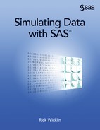
x = { 1 0, 1 1, -1 -1}; y = { 0 0, -1 0}; P = PairwiseDist(x, y); /* not printed */ D = EuclideanDistance(x); print D;
Figure A. 6 Distances between Two-Dimensional Points
A.9.2 The FROOT Function
The FROOT function numerically finds zeros of a univariate function. The BISECTION module implements some of the functionality of the FROOT function. To use the BISECTION module, the function whose root is desired must be named FUNC.
/* Bisection: find root on bracketing interval [a, b].
    If x0 is the true root, find c such that
    either |x0-c| < dx or |f(c)| < dy.
    You could pass dx and dy as parameters. */
start Bisection(a, b);
   dx = 1e-6; dy = 1e-4;
   do i = 1 to 100;                                     /* max iterations */
      c = (a+b)/2;
      if abs(Func(c)) < dy | (b-a)/2 < dx then
         return(c);
      if Func(a)#Func(c) > 0 then a = c;
      else b = c;
   end;
   return (.);                                          /* no convergence */
finish;

/* test it: Find q such that F(q) = target */
start Func(x) global(target);
   cdf = (x + x##3 + x##5)/3;
   return( cdf-target );
finish;
target = 0.5;                     /* global variable used by Func module */
q = Bisection(0, 1);              /* find root on interval [0, 1] */
print q;
Figure A.7 Using Bisection to Solve for a Quantile

A.9.3 The SQRVECH Function
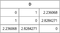
The SQRVECH function converts a symmetric matrix that is stored columnwise to a square matrix. The SQRVECH function is used in Section 8.5.2 and Section 10.4.2. The MYSQRVECH function duplicates the functionality of the SQRVECH function.
/* function that duplicates the SQRVECH function */
start MySqrVech(x);
   m = nrow(x)*ncol(x);
   n = floor( (sqrt(8*m+1)-1)/2 );
   if m ^= n*(n+1)/2 then do;
      print “Invalid length for input vector”; STOP;
   end;
   U = j(n, n, 0);
   col = repeat(1:nrow(U), nrow(U));
   row = T(col);
   idx = loc(row<=col);             /* indices of upper triangular matrix     */
   U[idx] = x;                      /* assign values to upper triangular      */
   L = T(U);                        /* copy to lower triangular               */
   idx = loc(row=col);              /* indices of diagonal elements           */
   L[idx] = 0;                      /* zero out diagonal for L                */
   return( U + L );                 /* return symmetric matrix                */
finish;

y = 1:15;
z = MySqrVech(y);
print z;
Figure A. 8 A Symmetric Matrix
A.9.4 The SAMPLE Function
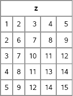
The SAMPLE function generates a random sample from a finite set. The SAMPLE function is used for bootstrapping in Section 15.5. The SAMPLEREPLACE module implements random sampling with replacement and equal probability. The SAMPLEREPLACE function returns an n × k matrix of elements sampled with replacement from a finite set.
/* Random sampling with replacement and uniform probability.
   Input: A is an input vector.
   Output: (n × k) matrix of random values from A. */
start SampleReplace(A, n, k);
   r = j(n, k);                         /* allocate result matrix   */
   call randgen(r, “Uniform”);          /* fill with random U(0, 1) */
   r = ceil(nrow(A)*ncol(A)*r);         /* integers 1, 2,…, ncol(A) */
   return(shape(A[r], n));              /* reshape and return       */
finish;

x = {A B C A A B};
call randseed(1);
s = SampleReplace(x, 3, 4);
print s;
Figure A. 9 Samples with Replacement
A.10 SAS/IML Modules for Sample Moments
This section includes modules for computing the sample skewness and excess kurtosis of a univariate sample.
proc iml;
/* Formulas for skewness and kurtosis from Kendall and Stuart (1969)
   The Advanced Theory of Statistics, Volume 1, p. 85.
*/
/* Compute sample skewness for columns of x */
start Skewness(x);
   n = (x^=.)[+,];                                         /* countn(x, “col”)   */
   c = x - x[:,];                                          /* x - mean(x)        */
   k2 = (c##2)[+,] / (n-1);                                /* variance = k2      */
   k3 = (c##3)[+,] # n / ((n-1)#(n-2));
   skew = k3 / k2##1.5;
   return( skew );
finish;

/* Compute sample (excess) kurtosis for columns of x */
start Kurtosis(x);
   n = (x^=.)[+ ,];                                        /* countn(x, “col”)    */
   c = x - x[:,];                                          /* x - mean(x)         */
   c2 = c##2;
   m2 = c2[+,]/n;                                          /* 2nd central moments */
   m4 = (c2##2)[+,]/n;                                     /* 4th central moments */

   k2 = m2 # n / (n-1);                                    /* variance = k2       */
   k4 = n##2 /((n-1)#(n-2)#(n-3)) # ((n+1)#m4 - 3*(n-1)#m2##2);
   kurtosis = k4 / k2##2;
   return( kurtosis );                                     /* excess kurtosis     */
finish;

/* for the Gamma(4) distribution, the skewness
   is 2/sqrt(4) = 1 and the kurtosis is 6/4 = 1.5 */
call randseed(1);
x = j(10000, 1);
call randgen(x, “Gamma”, 4);
skew = skewness(x);
kurt = kurtosis(x);
print skew kurt;
Figure A.10 Sample Skewness and Kurtosis

In many applications, several sample moments are needed for a computation or analysis. In these situations, it is more efficient to compute the first four moments in a single call, as follows:
/* Return 4 × p matrix, M, where
     M[1,] contains mean of each column of X
     M[2,] contains variance of each column of X
     M[3,] contains skewness of each column of X
     M[4,] contains kurtosis of each column of X */
start Moments(X);
   n = (x^=.)[+ ,];                               /* countn(x, “col”)      */
   m1 =x[:,];                                     /* mean(x)               */
   c = x-m1;
   m2 = (c##2)[+,]/n;                             /* 2nd central moments   */
   m3 = (c##3)[+,]/n                              /* 3rd central moments   */
   m4 = (c##4)[+,]/n                              /* 4th central moments   */

   M = j(4, ncol(X));
   M[1,] = m1;
   M[2,] = n/(n-1) # m2;                          /* variance              */
   k3 = n##2 /((n-1)#(n-2)) # m3;
   M[3,] = k3 / (M[2,])##1.5;                     /* skewness              */
   k4 = n##2 /((n-1)#(n-2)#(n-3)) # ((n+1)#m4 - 3*(n-1)#m2##2);
   M[4,] = k4 / (M[2,])##2;                       /* excess kurtosis       */
   return( M );
finish;
A.11 References
Wicklin, R. (2010), Statistical Programming with SAS/IML Software, Cary, NC: SAS Institute Inc.