Chapter 4

Simulating Data to Estimate Sampling Distributions

Contents

4.1 The Sampling Distribution of a Statistic

Chapter 2, “Simulating Data from Common Univariate Distributions,” shows how to simulate a random sample with N observations from a variety of standard distributions. This chapter describes how to simulate many random samples and use them to estimate the distribution of sample statistics. You can use the sampling distribution to compute p-values, standard errors, and confidence intervals, just to name a few applications.

In data simulation, you generate a sample from a population model. If you compute a statistic for the simulated sample, then you get an estimate of a population quantity. For example, Figure 4.1 shows a random sample of size 50 drawn from some population. The third quartile of the sample is shown as a vertical line. It is an estimate for the third quartile of the population.

Figure 4.1 Random Sample and Quartile Statistic

You can repeat this process by drawing another random sample of size 50 and computing another sample quartile. If you continue to repeat this process, then you will generate a slew of statistics, one for each random sample. In Figure 4.2, one of the samples has the quartile value 8.4, another sample has the quartile value 9.6, a third sample has the quartile value 6.9, and so on.

The union of the statistics is an approximate sampling distribution (ASD) for the statistic. This ASD is shown in the bottom graph of Figure 4.2, which shows a histogram for 1,000 statistics, each statistic being the third quartile for a random sample drawn from the population. The “width” of the ASD (for example, the standard deviation) indicates how much the statistic is likely to vary among random samples of the same size. In other words, the width indicates how much uncertainty to expect in an estimate due to sampling variability. In the figure, the standard deviation of the ASD is 0.7 and the interquartile range is 0.9.

The simulated sampling distribution is approximate because it is based on a finite number of samples. The exact sampling distribution requires computing the statistic for all possible samples of the given sample size. The shape of the sampling distribution (both exact and approximate) depends on the distribution of the population, the statistic itself, and the sample size. For some statistics, such as the sample mean, the theoretical sampling distribution is known. However, for many statistics the sampling distribution is known only by using simulation studies.

Figure 4.2 Accumulation of Many Statistics from Samples

The sampling distribution of a statistic determines a familiar statistic: the standard error. The standard error of a statistic is the standard deviation of its sampling distribution.

The sampling distribution is used to estimate uncertainty in estimates. It is also useful for hypothesis testing. Suppose that a colleague collects 50 observations and tells you that the third quartile of the data is 6, and asks whether you think it is likely that her data are from the population in Figure 4.2. From the figure, you notice that the statistic for her sample is smaller than all but a few of the simulated sample quartiles. Therefore, you respond that it is unlikely that her sample came from the population. This demonstrates the main idea of hypothesis testing: You look at some sampling distribution and compute the probability of a random value being at least as extreme as the value that you are testing. Hypothesis testing and p-values are discussed in Chapter 5, “Using Simulation to Evaluate Statistical Techniques.”

In summary, you can use simulation to construct an ASD for a statistic. The ASD enables you to compute quantities that are of statistical interest, such as the standard error and p-values for hypothesis tests.

4.2 Monte Carlo Estimates

The previous section describes the essential ideas of statistical simulation without using mathematics. This section uses statistical theory to describe the essential ideas. The presentation and notation are based on Ross (2006, p. 117–126), which is an excellent reference for readers who are interested in a more rigorous treatment of simulation than is presented in this book.

One use of simulation is to estimate some unknown quantity, θ, in the population by some statistic, X, whose expected value is θ. A statistic is a random variable. If you draw one sample from the population and compute the statistic, X₁, on that sample, then you have one estimate of θ. A second independent sample results in X₂, which is also an estimate of θ. After a large number (m) of samples, the union of the statistics is an approximation to the sampling distribution of X, given the population.

You can use the ASD of X to understand how the statistic can vary due to sampling variation. However, you can also use the ASD to form an improved estimate of θ. After m samples, you can compute the Monte Carlo estimate to θ, which is simply the average of the statistics: . The Monte Carlo estimate (like the X_i statistics) is an estimate of θ. However, it has a smaller variance than the X_i. The X_i have a common variance, σ², because they are random variables from the same population. To determine how close the Monte Carlo estimate is to θ, you can compute the mean square error, which is the expected value of ( − θ)². The mean square error equals σ²/m (Ross 2006, p. 118). The square root of this quantity, σ/, is a measure of how far the Monte Carlo estimate is from θ.

The Monte Carlo estimate, , is a good estimator of θ when σ/ is small. Of course, the population variance σ² is unknown, but is usually estimated by the sample variance S² = . The sample standard deviation S = is used to estimate σ.

You can use the Monte Carlo estimate to estimate discrete probabilities and proportions. An example is given in Section 4.4.3.

4.3 Approximating a Sampling Distribution

A statistical simulation consists of the following steps:

1. Simulate many samples, each from the same population distribution.
2. For each sample, compute the quantity of interest. The quantity might be a count, a mean, or some other statistic. The union of the statistics is an ASD for the statistic.
3. Analyze the ASD to draw a conclusion. The conclusion is often an estimate of something, such as a standard error, a confidence interval, a probability, and so on.

This chapter describes how to carry out this scheme efficiently in SAS software. This chapter focuses on simulating data from a continuous distribution and computing the ASD for basic statistics such as means, medians, quantiles, and correlation coefficients.

There are two main techniques for implementing step 1 and step 2: the BY-group technique and the in-memory technique.

BY-group technique: Use this technique when you plan to use a SAS procedure to analyze each sample in step 2. In this approach, you write all samples to the same data set. Each sample is identified by a unique value of a variable, which is called SampleID in this book. Use a BY statement in the SAS procedure to efficiently analyze each sample.

In-memory technique: Use this technique when you plan to use the SAS/IML language to analyze each sample in step 2.

• If you are analyzing univariate data, then it is common to store each simulated sample as a row (or column) of a matrix. You can then compute a statistic on each row (or column) to estimate the sampling distribution.
• If you are analyzing multivariate data, then it is common to write a DO loop. At each iteration, simulate data, compute the statistic on that data, and store the statistic in a vector. When the DO loop completes, the vector contains the ASD.

It is also possible to combine the techniques: If the simulated data are in a SAS data set but you intend to analyze the data in the SAS/IML language, you can read each BY group (sample) into a SAS/IML matrix or vector by using a DO loop and a WHERE clause in the READ statement.

4.4 Simulation by Using the DATA Step and SAS Procedures

This section provides several examples of using the DATA step to simulate data. The resulting data are analyzed by using SAS procedures, which compute statistics on the data by using the BY statement to iterate over all samples. The ASD of the statistic is analyzed by using a procedure such as PROC MEANS or PROC UNIVARIATE.

Each simulation in this chapter uses a fixed seed value so that you can reproduce the analysis and graphs. If you use a different value, then the graphs and analyses will change slightly, but the main ideas remain the same.

4.4.1 A Template for Simulation with the DATA Step and Procedures

To generate multiple samples with the DATA step, use the techniques that are described in Chapter 2, but put an extra DO loop around the statements that generate each sample. This outer loop is the simulation loop, and the looping variable identifies each sample. For example, suppose that you want to generate m samples, and each sample contains N observations. You can use the following steps to generate and analyze the simulated data:

1. Simulate data with known properties. The resulting data set contains N × m observations and a variable SampleID that identifies each sample. (Data that are arranged like this are said to be in the “long” format.) The SampleID variable must be in sorted order so that you can use it as a BY-group variable. If you generate the data in a different order, then sort the data by using the SORT procedure.
2. Use some procedure and the BY statement to compute statistics for each sample. Store the m results in an output data set.
3. Analyze the statistics in the output data set. Compute summary statistics and graph the approximate sampling distribution to answer questions about confidence intervals, hypothesis tests, and so on.

The following pseudocode is a template for these steps:

%let N = 10;                            /* size of each sample */
%let NumSamples = 100;                  /* number of samples   */ 
/* 1. Simulate data with DATA step */
data Sim;
do SampleID = 1 to &NumSamples;
   do i = 1 to &N;
      x = rand(“DistribName”, parami, param2, …);
      output;
   end;
end;
run;

/* 2. Compute statistics for each sample */
proc <NameOfProc> data=Sim out=OutStats noprint;
   by SampleID;
   /* compute statistics for each sample */
run;

/* 3. Analyze approx. sampling distribution of statistic */
proc univariate data=OutStats; /* or PROC MEANS or PROC CORR… */
   /* analyze sampling distribution */
run;

The Sim data set contains the SampleID variable, which has the values 1–100. The x variable contains random values from the specified distribution. The first 10 observations are the first simulated sample, the next 10 are the second sample, and so forth.

The second step (computing statistics and storing them in the OutStats data set) varies a little, depending on the procedure that you use to compute the statistics. There are four common ways to create the OutStats data set from a SAS procedure:

• By using an option in the PROC statement. For example, the OUTEST= option in the PROC REG statement creates an output data set that contains parameter estimates.
• By using an OUTPUT statement. For example, the MEANS procedure has an OUTPUT statement that writes univariate statistics to an output data set.
• By using an OUT= option in a procedure statement. For example, the TABLES statement in PROC FREQ has an OUT= option that writes frequencies and expected frequencies to an output data set.
• By using an ODS OUTPUT statement to write an ODS table to a data set.

The following sections apply this general template to specific examples. See Section 3.5 if you are not comfortable using ODS to select, exclude, and output tables and graphics.

4.4.2 The Sampling Distribution of the Mean

You can use a simple simulation to approximate the sampling distribution of the mean, which leads to an estimate for the standard error. This is a good example to start with because the sampling distribution of the mean is well known due to the central limit theorem (CLT). The CLT states that the sampling distribution of the mean is approximately normally distributed, with a mean equal to the population mean, μ, and a standard deviation equal to σ/, where σ is the standard deviation of the population (Ross 2006). This approximation gets better as the sample size, N, gets larger.

What is interesting about the CLT is that the result holds regardless of the distribution of the underlying population.

The following SAS statements generate 1,000 samples of size 10 that are drawn from a uniform distribution on the interval [0,1]. The MEANS procedure computes the mean of each sample and saves the means in the OutStatsUni data set.

%let N = 10;                            /* size of each sample */
%let NumSamples = 1000;                 /* number of samples   */
/* 1. Simulate data */
data SimUni;
call streaminit(123);
do SampleID = 1 to &NumSamples;
   do i = 1 to &N;
      x = rand(“Uniform”);
      output;
   end;
end;
run;

/* 2. Compute mean for each sample */
proc means data=SimUni noprint;
   by SampleID;
   var x;
   output out=OutStatsUni mean=SampleMean;
run;

The simulation generates the ASD of the sample mean for U(0,1) data with N = 10. The simulated sample means are contained in the variable SampleMean in the OutStatsUni data set. You can summarize the ASD by using the MEANS procedure (see Figure 4.3), and visualize it by using the UNIVARIATE procedure (see Figure 4.4), as follows:

/* 3. Analyze ASD: summarize and create histogram */
proc means data=OutStatsUni N Mean Std P5 P95;
   var SampleMean;
run;
ods graphics on;                             /* use ODS graphics   */
proc univariate data=OutStatsUni;
   label SampleMean = “Sample Mean of U(0,1) Data”;
   histogram SampleMean / normal;            /* overlay normal fit */
   ods select Histogram;
run;

Figure 4.3 Summary of the Sampling Distribution of the Mean of U(0,1) Data, N = 10

Figure 4.4 Approximate Sampling Distribution of the Sample Mean of U(0,1) Data, N = 10

Figure 4.3 shows descriptive statistics for the SampleMean variable. The Monte Carlo estimate of the mean is 0.5, and the standard error of the mean is 0.09. Figure 4.4 shows a histogram of the SampleMean variable, which appears to be approximately normally distributed.

You can use statistical theory to check whether the simulated values make sense. The U(0,1) distribution has a population mean of 1/2 and a population variance of σ² = 1/12. The CLT states that the sampling distribution of the mean is approximately normally distributed with mean 1/2 and standard deviation σ/ for large values of N. Even though N is small for this example, the standard deviation is nevertheless close to 1/ ≈ 0.0913.

The P5 and P95 options in the PROC MEANS statement make it easy to compute a 90% confidence interval for the mean. To compute a 95% confidence interval, use PROC UNIVARIATE to compute the 2.5 and 97.5 percentiles of the data, as follows:

proc univariate data=OutStatsUni noprint;
   var SampleMean;
   output out=Pctl95 N=N mean=Mean pctlpts=2.5 97.5 pctlpre=Pctl;
run;

proc print data=Pctl95 noobs;
run;

Figure 4.5 95% Confidence Intervals

Exercise 4.1: The standard exponential distribution has a mean and variance that are both 1. Generate 1,000 samples of size N = 64, and compute the mean and standard deviation of the ASD. Is the standard deviation close to 1/8?

4.4.3 Using a Sampling Distribution to Estimate Probability

Section 4.4.2 simulates samples of size N = 10 from a U(0,1) distribution. Suppose that someone draws a new, unseen, sample of size 10 from U(0,1). You can use the simulated results shown in Figure 4.4 to answer the following question: What is the probability that the mean of the sample is greater than 0.7?

You can write a short DATA step to compute the proportion of simulated means that satisfy this condition, as follows:

data Prob;
   set OutStatsUni;
   LargeMean = (SampleMean>0.7);      /* create indicator variable */
run;

proc freq data=Prob;
   tables LargeMean / nocum;          /* compute proportion        */
run;

Figure 4.6 Estimated Probability of a Mean Greater Than 0.7

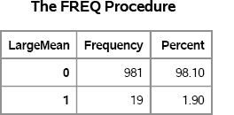
The answer is that only 1.9% of the simulated means are greater than 0.7. It is therefore rare to observe a mean this large in a random draw of size 10 from the uniform distribution.

Exercise 4.2: Instead of using the DATA step to create the LargeMean indicator variable, you can use the FORMAT procedure to define a SAS format that displays values that are less than 0.7 differently than values that are greater than 0.7, as follows:

proc format;
   value CutVal low-<0.7=“less than 0.7” 0.7-high=“greater than 0.7”;
run;

Use the CUTVAL. format to estimate the probability that SampleMean is greater than 0.7.

4.4.4 The Sampling Distribution of Statistics for Normal Data

This section generates data from the standard normal distribution and examines the sampling distributions of several statistics: the mean, the median, and the variance. Because the underlying distribution is normal, the following results are known (Kendall and Stuart 1977):

• Given a sample with an odd number of points, for example N = 2k + 1, the variance of the sample mean is about 64% smaller than the variance of the sample median. More precisely, the ratio of the variances is (4k)/(π(2k + 1)), which approaches 2/π ≈ 0.64 for large k.
• The sampling distribution of the variance follows a scaled chi-square distribution with N − 1 degrees of freedom.

This section shows you how to use statistical simulation to demonstrate these facts and, by extension, other “textbook facts” about the sampling distribution of statistics. The value of this section is that you can use these same techniques when no theoretical result is available.

When you use simulation to demonstrate a statistical fact about a sampling distribution, you need to simulate a large number of samples so that the ASD is a good approximation to the exact sampling distribution. The following statements generate 10,000 random samples from N(0,1), each of size N = 31 :

%let N = 31;               /* size of each sample */
%let NumSamples = 10000;   /* number of samples   */
/* 1. Simulate data */
data SimNormal;
call streaminit(123);
do SampleID = 1 to &NumSamples;
   do i = 1 to &N;
      x = rand(“Normal”);
      output;
   end;
end;
run;


/* 2. Compute statistics for each sample */
proc means data=SimNormal noprint;
   by SampleID;
   var x;
   output out=OutStatsNorm mean=SampleMean median=SampleMedian var=SampleVar;
run;

The program generates three sampling distributions: one for the mean, one for the median, and one for the variance. All three sampling distributions are stored in the OutStatsNorm data set.

4.4.4.1 Variance of the Sample Mean and Median

Each simulated sample has N = 31 observations. Let k = 15 so that N = 2k + 1. For these simulated data, is it true that the variance of the sample mean is (4k)/(π(2k + 1)) = 0.616 times the variance of the sample median? You can use PROC MEANS to compute the variances, which are shown in Figure 4.7.

/* variances of sampling distribution for mean and median */
proc means data=OutStatsNorm Var;
   var SampleMean SampleMedian;
run;

Figure 4.7 Variances of the Sample Mean and Median of N(0,1) Data

The simulation demonstrates that the theory works well. The ratio of the variances for the ASD in Figure 4.7 is 0.645, which is within 5% of the theoretical value.

It is interesting to overlay the two distributions to see how they compare. A simple way to compare two distributions is to plot their densities, as follows:

proc sgplot data=OutStatsNorm;

   title “Sampling Distributions of Mean and Median for N(0,1) Data”;
   density SampleMean / type=kernel legendlabel=“Mean”;
   density SampleMedian / type=kernel legendlabel=“Median”;
   refline 0 / axis=x;
run;

Figure 4.8 shows that the two distributions are approximately symmetric and have similar centers. However, the distribution of the median is wider, as predicted by theory.

Figure 4.8 Approximate Sampling Distribution for the Mean and Median of N(0,1) Data, N = 31

4.4.4.2 Sampling Distribution of the Variance

Statistical theory says that the quantity (N − 1)s²/σ² follows a chi-square distribution with N − 1 degrees of freedom, where s² is the sample variance and σ² is the variance of the underlying normal population. For the simulated data in this example, N = 31 and σ = 1.

You can use PROC UNIVARIATE to fit a chi-square distribution to the scaled sample variances. Fitting a parametric distribution to data is accomplished with the HISTOGRAM statement. A chi-square distribution with d degrees of freedom is equivalent to a Gamma(d/2,2) distribution. Therefore, the following statements fit a chi-square distribution to the scaled variances. The resulting histogram is shown in Figure 4.9.

/* scale the sample variances by (N-1)/sigma^2 */
data OutStatsNorm;
   set OutStatsNorm;
   ScaledVar = SampleVar * (&N-1)/1;
run;

/* Fit chi-square distribution to data */
proc univariate data=OutStatsNorm;
   label ScaledVar = “Variance of Normal Data (Scaled)”;
   histogram ScaledVar / gamma(alpha=15 sigma=2);   /* = chi-square */
   ods select Histogram;
run;

Figure 4.9 Scaled Distribution of Variance and Chi-Square Fit

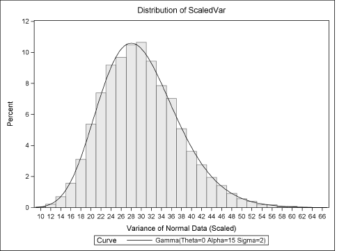
The goodness-of-fit statistics are not shown, but Figure 4.9 indicates that a Gamma(15, 2) distribution fits the sampling distribution. This is equivalent to a chi-square distribution with 30 degrees of freedom. This simulation agrees with the theoretical result that the variance of normal data follows a chi-square distribution.

4.4.5 The Effect of Sample Size on the Sampling Distribution

Section 4.4.2 demonstrates how to approximate the sampling distribution of the sample mean for samples of size 10 that are drawn from a uniform distribution. Statistical theory states that the sampling distribution of the sample mean is approximately normally distributed with mean 1/2 and standard deviation 1/.

You can use simulation to illustrate the effect of sample size on the standard deviation of the sampling distribution. The following simulation draws 1,000 samples of size 10, 30, 50, and 100, and displays the Monte Carlo estimates in Figure 4.10:

%let NumSamples = 1000;              /* number of samples */
/* 1. Simulate data */
data SimUniSize;
call streaminit(123);
do N = 10, 30, 50, 100;
   do SampleID = 1 to &NumSamples;
      do i = 1 to N;
         x = rand(“Uniform”);
         output;
      end;
   end;
end;
run;

/* 2. Compute mean for each sample */
proc means data=SimUniSize noprint;
   by N SampleID;
   var x;
   output out=OutStats mean=SampleMean;
run;

/* 3. Summarize approx. sampling distribution of statistic */
proc means data=OutStats Mean Std;
   class N;
   var SampleMean;
run;

Figure 4.10 Means and Standard Deviations of Sampling Distribution of the Mean

Notice that the simulation now includes the sample size, N, as a parameter that is varied during the simulation. There are actually four simulations being run, one for each sample size. The SAS syntax makes it easy to do the following:

• Simulate all of the data in a single DATA step by writing an extra DO loop outside of the usual simulation statements.
• Analyze all of the data by using both N and SampleID variables in the BY statement of the MEANS procedure.
• Display the mean and standard deviation of all the simulations by using the N variable in the CLASS statement in the second call to the MEANS procedure.

You can use the computed means and standard deviations to visualize the sampling distribution of the mean as the sample size increases. Figure 4.11 shows normal density distributions for the estimated parameters (μ_i, σ_i ), i = 1,…, 4.

Figure 4.11 Approximate Sampling Distribution of the Mean, N = 10, 30, 50,100

Exercise 4.3: Create Figure 4.11 by overlaying the normal PDFs whose parameters are given in Figure 4.10.

Exercise 4.4: The last column of Figure 4.10 shows that the standard error of the mean decreases as the sample size increases. Let the sample size, N, vary from 10 to 200 in increments of 10. Simulate 1,000 samples of size N from the uniform distribution. Plot the standard error of the mean as a function of the sample size.

4.4.6 Bias of Kurtosis Estimates in Small Samples

Although Section 4.4.1 shows how to write a DATA step that simulates data from a single distribution, you can easily extend the idea. This section uses a single DATA step to simulate data from four different distributions.

For small sample sizes drawn from distribution with large kurtosis, the sample kurtosis is known to underestimate the kurtosis of the population (Joanes and Gill 1998; Bai and Ng 2005). (Here “kurtosis” refers to “excess kurtosis”; see the discussion in Section 16.4.) In fact, Bai and Ng (2005, p. 49) comment:

Measuring the tails [of a distribution by] using the kurtosis statistic is not a sound approach…. The true value of [the kurtosis] will likely be substantially underestimated in practice, because a very large number of observations is required to get a reasonable estimate…. Exceptions are distributions with thin tails, such as the normal distribution.

Suppose that you want to run a simulation study to investigate the truth of the previous statement. You might choose a few distributions with known kurtosis, generate many small samples, compute the sample kurtosis for each sample, and compare the sample kurtosis to the known population value.

Table 4.1 shows the skewness and kurtosis for four distributions. The values for the lognormal distribution are approximate; the other values are exact.

Table 4.1 Skewness and Excess Kurtosis for Four Distributions

The following statements simulate 1,000 samples (each of size N = 50) from each distribution. PROC MEANS is used to compute the sample kurtosis and to save the values to the Moments data set.

/* bias of kurtosis in small samples */
%let N = 50;                         /* size of each sample */
%let NumSamples = 1000;              /* number of samples   */
data SimSK(drop=i);
call streaminit(123);
do SampleID = 1 to &NumSamples;      /* simulation loop             */
   do i = 1 to &N;                   /* N obs in each sample        */    
      Normal= rand(“Normal”);        /* kurt=0                      */
      t = rand(“t”, 5);              /* kurt=6 for t, exp, and logn */     
      Exponential = rand(“Expo”);     
      LogNormal = exp(rand(“Normal' , 0, 0.503));
      output;
   end;
end;
run;

proc means data=SimSK noprint;
   by SampleID;
   var Normal t Exponential LogNormal;
   output out=Moments(drop=_type_ _freq_) Kurtosis=;
run;

The KURTOSIS= option in the OUTPUT statement of PROC MEANS is used so that the kurtosis values in the Moments data set have the same names as the original variables. The following statements use PROC TRANSPOSE to transpose the data and PROC SGPLOT to create box plots of the four distributions. See Figure 4.12.

proc transpose data=Moments out=Long(rename=(col1=Kurtosis));
   by SampleID;
run;

proc sgplot data=Long;
   title “Kurtosis Bias in Small Samples: N=&N”;
   label _Name_ = “Distribution”;
   vbox Kurtosis / category=_Name_ meanattrs=(symbol=Diamond);
   refline 0 6 / axis=y;
   yaxis max=30;
   xaxis discreteorder=DATA;
run;

Figure 4.12 Distribution of Sample Kurtosis for Small Samples, N = 50

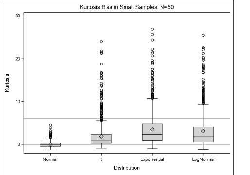
Figure 4.12 shows distributions of the sample kurtosis for small samples (N = 50) drawn from four different distributions. The mean value (the Monte Carlo estimate) is shown by a diamond. Horizontal reference lines are drawn to indicate the population kurtosis as shown in Table 4.1. For the normal distribution, the kurtosis sampling distribution is centered at 0, which is the value of the population kurtosis. However, the Monte Carlo estimates are less than the population value for the t, exponential, and lognormal distributions. Notice also that the distribution of the sample kurtosis is highly skewed and has a long tail.

The bias in the kurtosis estimate is less for large samples as shown in the following exercise.

Exercise 4.5: Repeat the simulation and redraw Figure 4.12 for samples that contain N = 2000 observations. Compare the range of sample kurtosis values for N = 50 and N = 2000.

Exercise 4.6: Is the skewness statistic also biased for small samples? Modify the example in this section to compute and plot the skewness of 1,000 random samples for N = 50. The skewness for each distribution is given in Table 4.1.

4.5 Simulating Data by Using the SAS/IML Language

This section shows how to simulate and analyze data by using the SAS/IML language. The first example simulates and analyzes univariate data; the second simulates multivariate data. The simulated samples and the ASD are analyzed by using SAS/IML functions.

4.5.1 The Sampling Distribution of the Mean Revisited

You can use SAS/IML software to repeat the simulation and computation in Section 4.4.3 and Section 4.4.5. The following program computes an ASD for the sample mean of U(0,1/ data (N = 10). Each sample is stored as a row of a matrix, x. This example shows an efficient way to simulate and analyze many univariate samples in PROC IML. The results of the program are shown in Figure 4.13.

%let N = 10;
%let NumSamples = 1000;
proc iml;
call randseed(123);
x = j(&NumSamples,&N)       /* many samples (rows), each of size N */
call randgen(x, “Uniform”)  /* 1. Simulate data                    */
s = x[,:];                  /* 2. Compute statistic for each row   */
Mean = mean(s);             /* 3. Summarize and analyze ASD        */
StdDev = std(s);
call qntl(q, s, {0.05 0.95});
print Mean StdDev (q`)[colname={“5th Pctl” “95th Pctl”}];

/* compute proportion of statistics greater than 0.7 */
Prob = mean(s > 0.7);
print Prob[format=percent7.2];

Figure 4.13 Analysis of the ASD of the Sample Mean of U(0,1/ Data, N = 10

Notice the following features of the SAS/IML program:

• There are no loops.
• Three statements are used to generate the samples: RANDSEED, J, and RANDGEN. A single call to the RANDGEN routine fills the entire matrix with random values.

In the program, the colon subscript reduction operator (:) is used to compute the mean of each row of the x matrix. The column vector s contains the ASD. The mean, standard deviation, and quantile of the ASD are computed by using the MEAN, STD, and QNTL functions, respectively. These functions operate on each column of their matrix argument. (Other SAS/IML functions that operate on columns include the MEDIAN and VAR functions.)

Figure 4.13 shows that the results are identical to the results in Figure 4.3 and Figure 4.6. The sampling distribution (not shown) is identical to Figure 4.4 because both programs use the same seed for the SAS random number generator and generate the same sequence of random variates. Notice that the SAS/IML program is more compact than the corresponding analysis that uses the DATA step and SAS procedures.

Notice that the PRINT statement prints the expression q`, which is read “q prime.” The prime symbol is the matrix transpose operator. It converts a column vector into a row vector, or transposes an N × p matrix into a p × N matrix. You can also use the T function to transpose a matrix or vector.

Exercise 4.7: Rewrite the simulation so that each column of x is a sample. The column means form the ASD. Use the T function, which transposes a matrix, prior to computing the summary statistics.

Exercise 4.8: Use the SAS/IML language to estimate the sampling distribution for the maximum of 10 uniform random variates. Display the summary statistics.

4.5.2 Reshaping Matrices

Exercise 4.7 shows that you can store each simulated sample in the column of a matrix. This is sometimes called the “wide” storage format. This storage format is useful when you intend to analyze each sample in SAS/IML software.

An alternative approach is to generate the data in SAS/IML software but to write the data to a SAS data set that can be analyzed by some other procedure. In this approach, you need to reshape the simulated data into a long vector and manufacture a SampleID variable that identifies each sample. This is sometimes called the “long” storage format. To represent the data in the long format, use the REPEAT and SHAPE function to generate the SampleID variable (see Appendix A, “A SAS/IML Primer”), as shown in the following statements:

proc iml;
call randseed(123);
x = j(&NumSamples,&N);   /* many samples (rows), each of size N    */
/* “long” format: first generate data IN ROWS… */
call randgen(x, “Uniform”);      /* 1. Simulate data (all samples) */
ID = repeat( T(1:&NumSamples), 1, &N); /* {1    1    …    1,
                                           2    2    …    2,
                                           …    …    …    …
                                         100  100    …  100} */
/* …then convert to long vectors and write to SAS data set */
SampleID = shape(ID, 0, 1);    /* 1 col, as many rows as necessary */
z = shape(x, 0, 1);
create Long var{SampleID z}; append; close Long;

The result of the SAS/IML program is a data set, Long, which is in the same format as the Sim data set that was created in Section 4.4.4. This trick works provided that the samples are stored in rows.

Actually, it is not necessary to reshape the matrices into vectors. The following statement also creates a data set with two columns. The data are identical to the Long data:

create Long2 var{ID x}; append; close Long2;

4.5.3 The Sampling Distribution of Pearson Correlations

When simulating multivariate data, each sample might be quite large. Rather than attempt to store all samples in memory, it is often useful to adopt a simulation scheme that requires less memory. In this scheme, only a single multivariate sample is ever held in memory.

To illustrate the multivariate approach to simulation in PROC IML, this example generates 20 random values from the bivariate normal distribution with correlation ρ = 0.3 by using the RANDNORMAL function, which is described in Section 8.3.1. Each call to the RANDNORMAL function returns a 20 × 2 matrix of ordered pairs from a correlated bivariate normal distribution. For each sample, the program computes the Pearson correlation between the variables.

%let N = 20;                      /* size of each sample            */
%let NumSamples = 1000;           /* number of samples              */
proc iml;
call randseed(123);
mu = {0 0}; Sigma = {1 0.3, 0.3 1};
rho = j(&NumSamples, 1);          /* allocate vector for results    */
do i = 1 to &NumSamples;          /* simulation loop                */
   x = RandNormal(&N, mu, Sigma); /* simulated data in N × 2 matrix */
   rho[i] = corr(x)[1,2];         /* Pearson correlation            */
end;
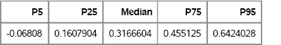
/* compute quantiles of ASD; print with labels */
call qntl(q, rho, {0.05 0.25 0.5 0.75 0.95});
print (q`)[colname={“P5” “P25” “Median” “P75” “P95”}];

Figure 4.14 Quantiles of the Approximate Sampling Distribution for a Pearson Correlation, N = 20

Each simulated sample consists of N observations and two columns and is held in the matrix x. Notice the DO loop. For each sample, the statistic (here, the correlation coefficient) is computed inside the DO loop and stored in the rho vector. During the next iteration, the x matrix is overwritten with a new simulated sample. This simulation scheme is often used for multivariate data. It requires minimal storage space (memory) but is less efficient because it is not vectorized as well as previous SAS/IML programs.

The result of this simulation shows that the sample correlation has a lot of variability for bivariate samples with 20 observations. As expected, the center of the sampling distribution is close to 0.3. However, 90% of the simulated correlations are in the interval [—0.07, 0.64], which is quite wide.

Descriptive statistics are useful for summarizing the ASD of a statistic such as the correlation coefficient, but a histogram is often more revealing. The following statements write the rho variable to a data set and call PROC UNIVARIATE to plot the histogram:

create corr var {“Rho”}; append; close;       /* write ASD */
quit;

/* 3. Visualize approx. sampling distribution of statistic */
ods graphics on;
proc univariate data=Corr;
   label Rho = “Pearson Correlation Coefficient”;
   histogram Rho / kernel;
   ods select Histogram;
run;

Figure 4.15 ASD of the Sample Correlation, Bivariate Data, N = 20, ρ = 0.3

The distribution of the correlation coefficient is not symmetric for this example. It has negative skewness.

Exercise 4.9: Use the ASD to estimate the probability that the sample correlation coefficient is negative for a sample of size 20 from the bivariate normal distribution in this section. (See Section 4.4.3.)

4.6 References

Bai, J. and Ng, S. (2005), “Tests for Skewness, Kurtosis, and Normality for Time Series Data,” Journal of Business and Economic Statistics, 23, 49–60.

Joanes, D. N. and Gill, C. A. (1998), “Comparing Measures of Sample Skewness and Kurtosis,” Journal of the Royal Statistical Society, Series D, 47, 183–189.

Kendall, M. G. and Stuart, A. (1977), The Advanced Theory of Statistics, volume 1, 4th Edition, New York: Macmillan.

Ross, S. M. (2006), Simulation, 4th Edition, Orlando, FL: Academic Press.