Chapter 15

Resampling and Bootstrap Methods

Contents

15.1 An Introduction to the Bootstrap

Bootstrap methods are nonparametric techniques that simulate data directly from a sample. These techniques are often used when no statistical model of the data is evident. Introductory references for bootstrap techniques include Efron and Tibshirani (1993) and Davison and Hinkley (1997).

Bootstrap methods use the fact that the empirical CDF (ECDF) of the data is an approximation to the underlying distribution. Consequently, the basic bootstrap method is essentially an inverse CDF technique (see Section 7.4.2) for sampling from the ECDF. The basic bootstrap technique is also called the simple bootstrap or the naive bootstrap.

This chapter presents efficient techniques for implementing the simple bootstrap in SAS software. This chapter also presents two variations of the simple bootstrap. The so-called parametric bootstrap is actually a classical technique that predates the introduction of the bootstrap. In the parametric bootstrap, you fit a parametric distribution to the data and then sample from this parametric distribution. The second variation is called the smooth bootstrap. In the smooth bootstrap, you randomly select observations from the data and add random noise.

The purpose of this chapter is to demonstrate a few basic techniques for bootstrapping. This chapter is far from comprehensive. See Cassell (2007) and Cassell (2010) for additional discussion of bootstrapping in SAS.

15.2 Resampling Techniques in SAS Software

There are three general techniques in SAS software for resampling data:

The DATA Step: You can use the POINT= option in the SET statement to randomly select observations from a SAS data set. For many data sets you can use the SASFILE statement to read the entire sample data into memory, which improves the performance of random access.

The SURVEYSELECT Procedure: You can use the SURVEYSELECT procedure to randomly select observations according to several sampling schemes.

SAS/IML Software: You can use built-in or user-defined functions to resample from the data.

This chapter uses a subset of Fisher's famous iris data to illustrate the bootstrap technique. Execute the following statements to generate the example data:

data Virginica(drop=Species);
set Sashelp.Iris(where=(Species=“Virginica”));
run;

The Virginica data contain measurements of 50 flowers of the species Iris virginica. The primary variable that is studied in this chapter is the SepalLength variable, which measures the length of the sepal (in millimeters) of each flower.

Suppose that you are interested in understanding the sampling variation for the skewness and kurtosis of the SepalLength variable. You can use PROC MEANS to compute point estimates, as shown in Figure 15.1.

proc means data=Virginica nolabels Skew Kurt;
   var SepalLength;
run;

Figure 15.1 Sample Skewness and Kurtosis

PROC MEANS does not support computing the standard error for these statistics, nor does it support confidence intervals for the parameters. However, you can use bootstrap methods to estimate these quantities. Implementing a bootstrap method requires three main steps:

1. Compute the statistic of interest on the original data, as in Figure 15.1.
2. Resample B times from the data to form B bootstrap samples.
3. Compute the statistic on each resample.

The statistics that are computed from the resampled data form a bootstrap distribution. The bootstrap distribution is an estimate of the sampling distribution of a statistic. In particular, the standard deviation of the bootstrap distribution is an estimate for the standard error of the statistic. Percentiles of the bootstrap distribution are a simple way to estimate confidence intervals.

Bootstrap confidence intervals are especially useful when the alternative approach produces a symmetric confidence interval such as ŝ ± z_α/2SE, where ŝ is a point estimate, z_α/2 is a standard normal quantile, and SE is an estimate of the standard error. These symmetric confidence intervals are often based on asymptotic normality of the sampling distribution of the statistic. For small samples, the distribution might not be symmetric, much less normally distributed. In general, bootstrap estimates of a confidence interval are not symmetric about the point estimate.

Step 1 of the algorithm is not strictly necessary, but it is useful for studying bias in the estimate. It is also used for permutation tests and hypothesis tests: a p-value for the observed statistic is estimated by using a bootstrap distribution that is generated by resampling according to the null hypothesis.

You can use many of the tips and techniques in this book to implement bootstrap methods in SAS software. The main difference between simulation and bootstrapping is that simulation draws random samples from a model of the population, whereas bootstrap samples are created by sampling with replacement directly from the data.

15.3 Resampling with the DATA Step

The simplest way to sample with replacement in the DATA step is to use the POINT= option in the SET statement. The following DATA step implements a resampling algorithm:

%let MyData = Virginica;
%let NumSamples = 5000;

sasfile &MyData load;                                  /* 1    */
data BootDS(drop=i);
call streaminit(1);
do SampleID = 1 to &NumSamples;                        /* 2    */
   do i = 1 to NObs;                                   /* 4    */
      choice = ceil(NObs * rand(“Uniform”));           /* 5    */
      set &MyData point=choice nobs=NObs;              /* 3, 6 */
      output;
   end;
end;
STOP;                                                  /* 7    */
run;
sasfile &MyData close;                       /* release memory */

The DATA step uses the following techniques, which are indicated by comments:

1. Provided that the data set is not too large, use the SASFILE statement to load the data into memory, which speeds up random access.
2. The SampleID variable is used to identify each sample.
3. SAS sets the value of the NObs variable to be the number of observations. This value is set before the DATA step runs. Consequently, the value of NObs is available throughout the DATA step, and in particular on statements that execute prior to the SET statement.
4. Randomly sample NObs observations.
5. Select a random integer in the range 1–NObs, as discussed in Section 2.4.4.
6. Use the POINT= option to read the selected observation.
7. Stop processing when all resamples are output.

The BootDS data set contains 5,000 samples, each with 50 observations. The samples are identified by the SampleID variable. This technique, in which an entire row is output at each iteration, is known as case resampling.

If you are interested only in one or two variables, then you can use a KEEP statement to output only certain variables. Alternatively, you can use an ARRAY statement to cache the observations for certain variables in an array. Random access of elements in an array is usually more efficient than random access of observations in a data set. To use this technique, you have to know how many observations are in the data set. The following DATA step stores that information in a macro variable:

data _null_;
   call symput(‘N’, NObs);
   if 0 then set &MyData nobs=NObs;
   STOP;
run;

The following DATA step resamples from the SepalLength variable 5,000 times. The main advantage over the previous method is that this technique reads each observation only once.

%let VarName = SepalLength;
data BootArray(keep= SampleID &VarName);
array arr_y[&N] _temporary_;

do i = 1 to NObs;                                    /* read data one time   */
   set &MyData point=i nobs=NObs;                    /* store obs in array   */
   arr_y[i] = &VarName;
end;

do SampleID = 1 to &NumSamples;                      /* resampling algorithm */
   do i = 1 to NObs;
      choice=ceil(NObs * rand(“Uniform”));

      &VarName = arr_y[choice];                      /* get value from array */
 
      output;
   end;
 
end;
STOP;
run;

The program uses an array to hold an entire variable in memory. This technique is easy to implement for one variable. The disadvantage of this method is that it is memory intensive and that you need an array for every variable that you want to bootstrap. (Alternatively, you could use a double array.)

You can use BY-group processing to analyze the BootDS or the BootArray data in the usual way. For example, the following statement computes the bootstrap estimates of skewness and kurtosis for the SepalLength variable:

/* compute bootstrap estimate on each bootstrap sample */
proc means data=BootDS noprint;
   by SampleID;
   var SepalLength;
   output out=OutStats skew=Skewness kurt=Kurtosis;
run;

The OutStats data set contains 5,000 observations. Each observation is the sample skewness and kurtosis of one of the bootstrap resamples. The union of these statistics is the bootstrap distribution of the statistic. The following statements construct a scatter plot that shows the joint distribution of the sample skewness and kurtosis on the bootstrap resamples:

proc sgplot data=OutStats;
   title “Bootstrap Estimates of Skewness and Kurtosis”;
   scatter x=Skewness y=Kurtosis / transparency=0.7;
   refline 0.118 / axis=x;     /* reference line at observed values */
   refline 0.033 / axis=y;
   label Skewness= Kurtosis=;
run;

Figure 15.2 Bootstrap Distribution of the Sample Skewness and Kurtosis

You can also request summary statistics for the bootstrap distribution. The mean is the bootstrap estimate of the parameter. The standard deviation is the bootstrap estimate for the standard error. The α/2 and 1 – α/2 quantiles of the bootstrap distribution form an approximate 100(1 – α)% confidence interval. The P5 and P95 options in the PROC MEANS statement make it easy to compute a 90% confidence interval, as shown in Figure 15.3.

proc means data=OutStats nolabels N Mean StdDev P5 P95;
   var Skewness Kurtosis;
run;

Figure 15.3 Descriptive Statistics for Skewness and Kurtosis

To compute a 95% confidence interval, use PROC UNIVARIATE to compute the 2.5 and 97.5 percentiles of the data, as shown in the following statements. The result is shown in Figure 15.4.

proc univariate data=OutStats noprint;
   var Skewness Kurtosis;
   output out=Pctl95 pctlpts =2.5  97.5   pctlname=P025 P975
                 pctlpre =Skew_ Kurt_ mean=SkewMean KurtMean;
run;

proc print data=Pctl95 noobs; run;

Figure 15.4 Means and 95% Confidence Intervals

Exercise 15.1: Draw histograms of the bootstrap distributions of the skewness and kurtosis.

Exercise 15.2: The following statements define a macro variable that records the elapsed time:

%let t0 = %sysfunc(datetime());
   /* put computation here */
%let t1 = %sysfunc(datetime());
%let elapsedTime = %sysevalf(&t1-&t0);

Compare the times for each DATA step technique to generate 5,000 resamples of the Virginica data.

15.4 Resampling with the SURVEYSELECT Procedure

The previous section shows that for the simplest sampling scheme (sampling with replacement), it is easy to use the DATA step to program a resampling scheme. However, experienced SAS programmers use the SURVEYSELECT procedure for resampling from data for the following reasons:

• It is about as fast as the DATA step array method.
• It supports many sampling schemes and can be used for jackknife methods.
• It requires no programming.
• It manufactures a frequency variable, which can decrease the size of the output data set.

For moderate size data, use the SASFILE statement (see Section 15.3) to load the data into RAM. This technique is not shown for the example in this section.

15.4.1 Resampling without Creating a Frequency Variable

The following statements, which are described later, use PROC SURVEYSELECT to generate 5,000 resamples of observations in the Virginica data set, which was created in Section 15.2:

%let MyData = Virginica;
%let NumSamples = 5000;
proc surveyselect data=&MyData NOPRINT seed=1          /* 1 */
     out=BootSS(rename=(Replicate=SampleID))           /* 2 */
     method=urs samprate=1                             /* 3 */
     reps=&NumSamples                                  /* 4 */
     outhits;                                          /* 5 */
run;

The call to PROC SURVEYSELECT does the following:

1. The SEED= option specifies the seed value for random number generation. If you specify a zero seed, then omit the NOPRINT option so that the value of the chosen seed appears in the procedure output.
2. The BY-group variable in the output data set is named Replicate. For consistency, rename this variable to SampleID.
3. The METHOD=URS option specifies unrestricted random sampling, which means sampling with replacement and with equal probability. The SAMPRATE=1 option specifies that each resample is the same size as the original data.
4. The REPS= option specifies how many bootstrap resamples you want to generate.
5. The OUTHITS options specifies that the output data set contains N × NumSamples observations, where N is the number of observations in the original data set (assuming that SAMPRATE=1). If a record is selected three times, then the output data set contains three (consecutive) copies of that record. In contrast, if you omit the OUTHITS option, then the output data set has fewer observations and the NumberHits variable contains the number of times that each record was selected. Consequently, you can refer to the NumberHits variable in the FREQ (or WEIGHT) statement of procedures that support the FREQ statement.

The following statements create bootstrap distributions for the skewness and kurtosis. The MEANS procedure produces Figure 15.5, which shows the mean, standard deviation, and middle 90% interval for the bootstrap distribution for the skewness and kurtosis. Compare these values with Figure 15.3.

proc means data=BootSS noprint;
   by SampleID;
   var SepalLength;
   output out=OutStats skew=Skewness kurt=Kurtosis;
run;

proc means data=OutStats nolabels N Mean StdDev P5 P95;
   var Skewness Kurtosis;
run;

Figure 15.5 Descriptive Statistics for Bootstrap Distributions

15.4.2 Resampling and Creating a Frequency Variable

You can reduce the size of the output data set by omitting the OUTHITS option in the SURVEYSELECT procedure. If you omit the option, then the NumberHits variable in the output data set contains the frequency for each observation. Consequently, you can analyze the output data as follows:

proc surveyselect data=&MyData NOPRINT seed=1
     out=BootSSFreq(rename=(Replicate=SampleID))
     method=urs samprate=1 reps=&NumSamples;
run;

proc means data=BootSSFreq noprint;
   by SampleID;
   freq NumberHits;
   var SepalLength;
   output out=OutStats2 skew=Skewness kurt=Kurtosis;
run;

Exercise 15.3: Run the preceding statements. Analyze the bootstrap distributions and compare your results with Figure 15.5. Do you obtain the same results if you use the same SEED= option?

15.5 Resampling Univariate Data with SAS/IML Software

SAS/IML 12.1 supports the SAMPLE function (see Section 2.6.2) that you can use to sample (with or without replacement) from a finite set. Prior to SAS/IML 12.1, you can use the SAMPLEREPLACE module, which is included in Appendix A. The following SAS/IML program uses the SKEWNESS and KURTOSIS modules, which are defined in Appendix A, to compute the bootstrap distributions for the skewness and kurtosis of the SepalLength variable. The bootstrap estimates are shown in Figure 15.6. They are similar to the estimates given in Figure 15.5. The SAS/IML QNTL function can compute any quantile, so you can use the parameters {0.025 0.975} to obtain a 95% confidence interval.

%let MyData = Virginica;
%let NumSamples = 5000;

/* Basic bootstrap to explore variation of skewness and kurtosis */
proc iml;
call randseed(12345);
load module=(Skewness Kurtosis); /* load SampleReplace if necessary */
use &MyData;
read all var {SepalLength} into x;
close &MyData;

/* get all bootstrap resamples with a single call */
/* s = SampleReplace(x, nrow(x), &NumSamples); */  /* prior to 12.1 */
s = sample(x, &NumSamples // nrow(x));      /* 50 × NumSamples      */
M = Skewness(s) // Kurtosis(s);             /* bootstrap statistics */
M = M` ;                                     /* NumSamples × 2      */

means = mean(M);                /* summarize bootstrap distribution */
call qntl(q, M, {0.05 0.95});
s = means` || q`;
VarNames = {“Skewness” “Kurtosis”};
StatNames = {“Mean” “P5” “P95”};
print s[format = 9.5 r=VarNames c=StatNames];

Figure 15.6 Means and Confidence Intervals, Computed in PROC IML

15.6 Resampling Multivariate Data with SAS/IML Software

The previous section constructs bootstrap samples of a single variable and uses the samples to construct the bootstrap distribution of the skewness and kurtosis statistics. This is done without writing a single loop. The program uses a SAS/IML matrix to hold all of the bootstrap samples, one in each column. The SAS/IML language enables you to compute the sample skewness and kurtosis statistics for each column in a vectorized manner.

As discussed in Section 4.5.3, if you are generating multivariate samples, then it is often convenient to write a loop. Inside the loop you generate each multivariate sample and compute the corresponding statistic.

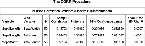
To illustrate this technique, consider the task of bootstrapping the correlation coefficients for the SepalLength, SepalWidth, and PetalLength variables in the Virginica data set. The goal is to estimate the distribution of the correlation coefficients, including a 95% confidence interval. As a check, you can use PROC CORR and Fisher's z transformation to generate the sample correlation and the 95% confidence intervals, which are shown in Figure 15.7:

/* compute sample correlations and Fisher 95% CI */
proc corr data=&MyData noprob fisher(biasadj=no);
   var SepalLength SepalWidth PetalLength;
   ods select FisherPearsonCorr;
run;

Figure 15.7 Sample Correlation Coefficients and 95% Confidence Intervals

You can use bootstrap methods to approximate the sampling distribution for the correlation coefficients. Each bootstrap sample is a 50 × 3 matrix that is generated by resampling with replacement from the 50 rows in the data. For each sample, you can compute the Pearson correlation coefficients for the three variables. The following SAS/IML program stores the correlation coefficients in rows of the rho matrix. Figure 15.8 displays some descriptive statistics for the bootstrap distributions.

/* bootstrap of MV samples */
proc iml;
call randseed(12345);
use &MyData;
read all var {“SepalLength” “SepalWidth” “PetalLength”} into X;
close &MyData;

/* Resample from the rows of X. Generate the indices for
   all bootstrap resamples with a single call */
N = nrow(X);
/* ndx = SampleReplace(1:N, &NumSamples, N); */
ndx = Sample(1:N, N // &NumSamples);        /* NumSamples × N       */

rho = j(&NumSamples, ncol(X));     /* allocate for results          */
do i = 1 to &NumSamples;
   rows = ndx[i, ];                /* selected rows for i_th sample */
   Y = X[rows, ];                  /* the i_th sample               */
   c = corr(Y);                    /* correlation matrix            */
rho[i, ] = c[{2 3 6}]';            /* upper triangular elements     */
end;

means = mean(rho);                 /* summarize bootstrap distrib   */
call qntl(q, rho, {0.025 0.975});
s = means` || q`;
varNames = {“p12” “p13” “p23”};
StatNames = {“Mean” “P025” “P975”};
print s[format = 9.5 r=VarNames c=StatNames];

Figure 15.8 Bootstrap Estimates of Correlations and 95% Confidence Intervals

The means of the bootstrap distributions are close to the sample correlations, which are shown in Figure 15.7. The confidence intervals are also close to the Fisher confidence limits. The main difference is the wider confidence interval for p23, which is the correlation between SepalWidth and PetalLength.

Exercise 15.4: Write the rho matrix to a SAS data set and use the MATRIX statement in the SGSCATTER procedure to visualize the joint distribution of the correlation coefficients. Use the DIAGONAL= option to add histograms and kernel density estimates for each correlation coefficient.

15.7 The Parametric Bootstrap Method

What some people call the parametric bootstrap is nothing more than the process of fitting a model distribution to the data and simulating data from the fitted model.

The first step is to choose a model for the data. If you have domain-specific knowledge of the process that generates the data, then that knowledge might suggest a model. For example, exponential models and Poisson models are often chosen because you assume that some process occurs at a constant rate.

If you do not have domain-specific knowledge, then choosing a distribution that models the data can be difficult. Chapter 16 describes how to use the moment-ratio diagram to choose candidate distributions from common “named” distributions. Alternatively, the same chapter describes how to use moment-matching to construct a distribution that matches the first four central moments of the sample data.

After you choose a model, you can use various SAS procedures to fit the model parameters. For continuous univariate data, PROC UNIVARIATE supports fitting a variety of common distributions. See Section 16.6 for an example. For more sophisticated models, there are many SAS procedures that fit parameters to data including PROC MODEL in SAS/ETS software and PROC NLIN in SAS/STAT software.

The last step is simulation from the model, which is discussed throughout this book.

15.8 The Smooth Bootstrap Method

In Section 15.4, the BootSS data set was created, which contains 5,000 resamples from the Virginica data. The following statements plot the bootstrap distribution for the median of the SepalLength variable. The distribution is shown in Figure 15.9.

proc means data=BootSS noprint;
   by SampleID;
   var SepalLength;
   output out=OutMed median=Median;
run;

proc univariate data=OutMed;
   histogram Median / kernel;
   ods select histogram;
run;

Figure 15.9 Bootstrap Distribution of the Sample Median

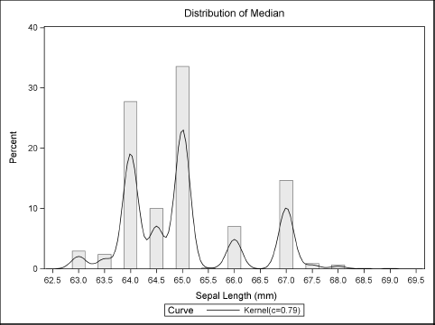
Figure 15.9 shows that the bootstrap distribution for the median is not continuous. However, the true sampling distribution of the median is continuous, so what is going on?

The problem is that the median (or any quantile) of a bootstrap resample can only attain a small number of values. For a sample of size N, it is a combinatorial fact that the bootstrap median can only assume at most 2N – 1 possible values: the N sample values and the N — 1 midpoints between adjacent ordered values. In practice, the bootstrap median attains a small number of possible values determined by data values near the sample median, as shown in Figure 15.9.

One way to overcome this problem is to add a small amount of random noise to each data point that is selected during the bootstrap resampling. This is equivalent to sampling from a kernel density estimate rather than sampling from the ECDF.

The question arises, if you intend to add a random quantity of the form ∊_i ~ N(0, λ), where λ is the standard deviation parameter, then what value should you choose for λ? Some researchers suggest choosing λ to be an estimate of the standard error of the statistic. Others might prefer to use the bandwidth of the kernel density estimate of the original data.

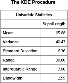
A bootstrap estimate of the standard error of the median is about 1.11. Because the UNIVARIATE procedure reports a standardized bandwidth, the following statements use PROC KDE to compute the bandwidth. See Figure 15.10.

%let MyData = Virginica;
%let VarName = SepalLength;
proc kde data=&MyData;
   univar SepalLength / method=SJPI unistats;
   ods select UnivariateStatistics;
run;

Figure 15.10 Summary Statistics and Bandwidth for Sample Data

Regardless of how you obtain a value for λ, the smooth bootstrap proceeds as follows. If the data value x_i, is selected for inclusion into a bootstrap sample, then use the value x_i + ∊_i, where ∊_i ~ N(0, λ). The following SAS/IML program implements the smooth bootstrap method:

proc iml;
/* Smooth bootstrap.
   Input: A is an input vector with N elements.
   Output: (B × N) matrix. Each row is a sample.
   Prior to SAS/IML 12.1, use the SampleReplace module */ 
start SmoothBootstrap(x, B, Bandwidth);
   N = nrow(x) * ncol(x);
   /* s = SampleReplace(x, B, N); */       /* prior to SAS/IML 12.1 */
   s = Sample(x, N // B);                        /* B x N matrix    */
   eps = j(B, N);                                /* allocate vector */
   call randgen(eps, “Normal”, 0, Bandwidth);    /* fill vector     */
   return( s + eps );                            /* add random term */
finish;

You can call the SMOOTHBOOTSTRAP module on the SepalLength variable in the Virginica data. The SMOOTHBOOTSTRAP module returns each bootstrap sample in a row, so transpose the return value before computing the median. The following program uses the Sheather-Jones bandwidth estimate (λ = 2.59) that is shown in Figure 15.10 to produce the histogram that is shown in Figure 15.11. Compare Figure 15.11 with Figure 15.9. The smooth bootstrap is a much better estimate of the sampling distribution of the median.

use &MyData; read all var {SepalLength} into x; close &MyData;

call randseed(12345);
y = SmoothBootstrap(x, &NumSamples, 2.59);        /* SJPI bandwidth */
Median = Median(y'),                  /* smooth bootstrap estimates */
create Smooth var {“Median”}; append; close Smooth;
quit;

proc univariate data=Smooth;
   histogram Median / kernel;
   ods select histogram;
run;

Figure 15.11 Smooth Bootstrap Distribution of the Sample Median

Exercise 15.5: Implement the smooth bootstrap in the DATA step by adding a small random normal variate to each observation in the OutMed data set, which is created in Section 15.4.

15.9 Computing the Bootstrap Standard Error

The bootstrap standard error is estimated by computing the standard deviation of the bootstrap distribution. The usual sample estimate of variance has a divisor of N – 1 for a sample of size N. However, the bootstrap estimate of variance requires using N as a divisor (Davison and Hinkley 1997). This means that to compute a bootstrap estimate of the variance of a statistic (or any related statistic, such as a Student's t confidence interval), then you need to estimate the variance by using a slightly different formula.

Both PROC MEANS and PROC UNIVARIATE support a VARDEF= option in the PROC statement. The default value is VARDEF=DF, which results in a variance divisor of N – 1. You can correct the variance estimate by multiplying it by the factor (N – 1)/N. Alternately, you can use the VARDEF=N option.

15.10  Computing Bootstrap Confidence Intervals

In this chapter, simple quantiles of the bootstrap distribution are used to construct confidence intervals. (For a significance level α, a basic confidence interval is formed from the α/2 and 1 – α/2 quantiles.) This simple method performs well for quantiles and for unbiased statistics.

However, for biased statistics, the simple method amplifies the bias. There are popular techniques that can be used to correct for bias (Efron and Tibshirani 1993). The bias-corrected (BC) confidence intervals adjust the quantiles. That is, instead of using the α/2 and 1 – α/2 quantiles, new quantiles are computed that depend on the estimate of the bias. Another technique is the bias-corrected and accelerated (BC_a) confidence interval. A good overview and discussion of these techniques are available in the article, comments, and rejoinder by DiCiccio and Efron (1996).

In SAS, several bootstrap techniques are provided by a series of macros that are provided by SAS. The %BOOT and %BOOTCI macros provide bootstrap methods and several kinds of confidence intervals. These macros and documentation are available at support.sas.com/kb/24/982.html.

15.11  References

Cassell, D. L. (2007), “Don't Be Loopy: Re-sampling and Simulation the SAS Way,” in Proceedings of the SAS Global Forum 2007 Conference, Cary, NC: SAS Institute Inc.
URL http://www2.sas.com/proceedings/forum2007/183-2007.pdf

Cassell, D. L. (2010), “BootstrapMania!: Re-sampling the SAS Way,” in Proceedings of the SAS Global Forum 2010 Conference, Cary, NC: SAS Institute Inc.
URL http://support.sas.com/resources/papers/proceedings10/268-2010.pdf

Davison, A. C. and Hinkley, D. V. (1997), Bootstrap Methods and Their Application, Cambridge: Cambridge University Press.

DiCiccio, T. J. and Efron, B. (1996), “Bootstrap Confidence Intervals,” Statistical Science, 11, 189–212.

Efron, B. and Tibshirani, R. J. (1993), An Introduction to the Bootstrap, New York: Chapman & Hall.