Chapter 7

Advanced Simulation of Univariate Data

Contents

7.1 Overview of Advanced Univariate Simulation

Chapter 2, “Simulating Data from Common Univariate Distributions,” describes how to simulate data from a variety of discrete and continuous “named” distributions, such as the binomial, geometric, normal, and exponential distributions. This chapter explains how to simulate data from less commonly encountered univariate distributions and distributions with more complex structures.

7.2 Adding Location and Scale Parameters

You can add a location and a scale parameter to any distribution without changing its shape. If F is the (cumulative) distribution function of a random variable X, then the random variable Y = θ + σX for σ > 0 has the distribution function F((x – θ)/σ). If X has density function f, then Y has density (1/σ)f((x – θ)/σ) (Devroye 1986, p. 12). The parameter θ is a location parameter, whereas σ is a scale parameter. Parameters that are invariant under translation and scaling are called shape parameters.

In SAS 9.3, some SAS functions do not support a location or scale parameter for a distribution. For example, a general form for the density of the exponential distribution is f (x; θ, σ) = (1/σ) exp(–(x – θ)/σ) for x > θ, where θ is a location parameter and σ > 0 is a scale parameter. This is the form supported by the UNIVARIATE procedure. However, the exponential distribution is parameterized in three other ways in SAS software:

• The RAND function does not support location or scale. The RAND function uses the standardized density f (x; 0, 1) = e^–x.
• The PDF, CDF, and QUANTILE functions do not support a location parameter. The exponential density used by these functions is f (x ; 0, σ) = (1/σ) exp(–x/σ).
• The MCMC procedure supports the density f (x; 0,1/λ) = λe^–λx, where λ > 0 is a rate parameter.

Fortunately, you can include location and scale parameters even when a function does not explicitly support them:

• To simulate a random variate Y with location parameter θ and scale parameter σ, use the RAND function to generate the standard random variate X and form Y = θ + σX.
• To compute a PDF that incorporates location and scale, call the PDF function as (1/sigma) * PDF(“DistribName”, (x-theta)/sigma).
• To compute a CDF that incorporates location and scale, call the CDF function as CDF(“DistribName”, (x-theta)/sigma).
• To compute a quantile that incorporates location and scale, call the QUANTILE function as x = theta + sigma*QUANTILE(“DistribName”, p), where p is the probability such that P(X ≤ x) = p.
• To incorporate a rate parameter, define the scale parameter as σ = 1/λ.

SAS software provides about two dozen “named” distributions as listed in Section 2.7. For a few distributions, additional parameters are sometimes needed. The following list shows how to generate random variates with parameters that are not supported by the RAND function. The symbol ~ means “is distributed according to.” For example, X ~ N(0,1) means that the random variable X follows a normal distribution with mean 0 and unit standard deviation.

Exponential: The RAND function generates E ~ Exp(1). The random variable σE is an exponential random variable with scale parameter σ. The random variable E/λ is an exponential random variable with rate parameter λ.

Gamma: The RAND function generates G ~ Gamma(α). The random variable σG is a gamma random variable with scale parameter σ.

Lognormal: The RAND function generates N ~ N(μ, σ). The random variable exp(N) is lognormally distributed with parameters μ and σ.

Uniform: The RAND function generates U ~ U(0,1). The random variable a + (b – a)U is uniformly distributed on the interval (a, b).

For the lognormal distribution, notice that the location and scale parameters are added before the exponential transformation is applied.

Exercise 7.1: Simulate 1,000 exponential variates with scale parameter 2. Overlay the corresponding PDF. Compute the sample median. Is it close to the theoretical value, which is 2 ln(2) ≈ 1.386?

Exercise 7.2: Simulate 1,000 lognormal variates by simulating Y ~ N(1.5, 3) and applying the transformation X = exp(Y). Use PROC UNIVARIATE to verify that X is lognormally distributed with parameters 1.5 and 3.

7.3 Simulating from Less Common Univariate Distributions

You can often use random variates from simple distributions (in particular, the normal, exponential, and uniform distributions) to simulate data from more complicated distributions.

To illustrate this approach, this section shows how to simulate data from the Gumbel, inverse Gaussian, Pareto, generalized Pareto, power function, Rayleigh, Johnson S_B, and Johnson S_U distributions. Most of these distributions are supported by PROC UNIVARIATE, but they are not supported by the RAND function in SAS 9.3.

To simulate from other distributions, see the algorithms in Devroye (1986) and the “Details” section of the PROC MCMC documentation in the SAS/STAT User's Guide.

7.3.1 The Gumbel Distribution

The Gumbel distribution is sometimes called the Type I extreme value distribution (Johnson, Kotz, and Balakrishnan 1994, p. 686). It is the limiting distribution of the greatest value among n independent random variables, as n → ∞. The density function for the Gumbel distribution with location μ and scale σ is

To simulate data from a Gumbel distribution, let E ~ Exp(1) and form X = μ + σ(–log(E))(Devroye 1986, p. 414), as follows:

/* Simulate from Gumbel distribution (Devroye, p. 414) */
E = rand(“Exponential”);
x = mu + sigma*(-log(E));

7.3.2 The Inverse Gaussian Distribution

The inverse Gaussian distribution (also called the Wald distribution) describes the first-passage time of Brownian motion with positive drift. The UNIVARIATE procedure supports fitting an inverse Gaussian distribution with a location parameter, μ > 0, and a shape parameter, λ > 0. The density function for x > 0 is

The RANDGEN function in SAS/IML 12.1 software supports simulating data from the inverse Gaussian distribution. However, the RAND function in SAS 9.3 software does not. For completeness, the following DATA step simulates inverse Gaussian data. The algorithm is from Devroye (1986, p. 149), which shows how to use normal and uniform variates to simulate data from an inverse Gaussian distribution.

/* Simulate from inverse Gaussian (Devroye, p. 149) */
data InvGauss(keep= X);
mu =1.5;                              /* mu > 0      */
lambda =2;                            /* lambda > 0 */
c = mu/(2 * lambda);
call streaminit(1);
do i = 1 to 1000;
   muY = mu * rand(“Normal”)**2;      /* or mu*rand(“ChiSquare”, 1) */
   X = mu + c*muY - c*sqrt(4*lambda*muY + muY**2);
   /* return X with probability mu/(mu+X);  otherwise mu**2/X */
   if rand(“Uniform”) > mu/(mu+X) then /* or rand(“Bern”, X/(mu+X)) */
      X = mu*mu/X;
   output;
end;
run;

7.3.3 The Pareto Distribution

The RANDGEN function in SAS/IML 12.1 software supports simulating data from the Pareto distribution. The Pareto distribution with shape parameter a > 0 and scale parameter is k > 0 has the following density function for x > k:

In SAS 9.3, the RAND function does not support the Pareto distribution. The CDF for the Pareto distribution is F(x) = 1 – (k/x)^a; therefore, you can use the inverse CDF method (see Section 7.4) to simulate random variates (Devroye 1986, p. 29), as shown in the following DATA step:

/* Simulate from Pareto (Devroye, p. 29) */
data Pareto(keep= X);
a = 4;                    /* alpha > 0                               */
k = 1.5;                  /* scale > 0 determines lower limit for x */
call streaminit(1);
do i = 1 to 1000;
   U = rand(“Uniform”);
   X = k / U**(1/a);
   output;
end;
run;

The algorithm uses the fact that if U ~ U(0,1), then also (1 – U) ~ U(0,1).

7.3.4 The Generalized Pareto Distribution

The generalized Pareto distribution has the following cumulative distribution:

F(z; α) = 1 – (1 – αz)^1/α

where α is the shape parameter and z = (x – θ)/σ is a standard variable. (In spite of its name, there is not a simple relationship between these parameters and the parameters of the usual Pareto distribution.) You can use the inverse CDF algorithm (see Section 7.4) to simulate random variates. In particular, let U ~ U(0,1) be a uniform variate. Then Z = – (1/α)(U^α – 1) is a standardized generalized Pareto variate. Equivalently, the following statements simulate a generalized Pareto variate:

/* Generalized Pareto(threshold=theta, scale=sigma, shape=alpha) */
U = rand(“Uniform”);
X = theta - sigma/alpha * (U**alpha-1);

The algorithm uses the fact that if U ~ U(0,1), then also (1 – U) ~ U(0,1).

7.3.5 The Power Function Distribution

The power function distribution with threshold parameter θ, scale parameter σ, and shape parameter α has the following density function for θ < x < θ + σ:

If E ~ Exp(1), then Z = (1 – exp(–E))^1/α follows a standard power function distribution (Devroye 1986, p. 262). In the general case, you can simulate a random variate that follows the power function distribution by using the following statements:

   /* power function(threshold=theta, scale=sigma, shape=alpha) */
   E = rand(“Exponential”);
   X = theta + sigma*(1-exp(-E))**(1/alpha);

7.3.6 The Rayleigh Distribution

The Rayleigh distribution with threshold parameter θ and scale parameter σ has the following density function for x ≥ θ:

The Rayleigh distribution is a special case of the Weibull distribution. A Rayleigh random variable with scale parameter is the same as a Weibull random variable with shape parameter 2 and scale parameter Consequently, the following statement generates a random variate from the Rayleigh distribution:

   /* Rayleigh(threshold=theta, scale=sigma) */
   X = theta + rand(“Weibull”, 2, sqrt(2)*sigma);

Alternatively, you can use the inverse CDF method (Devroye 1986, p. 29).

7.3.7 The Johnson S_B Distribution

The Johnson system of distributions (Johnson 1949) is described in Section 16.7 and in the PROC UNIVARIATE documentation. The Johnson system is a flexible way to model data (Bowman and Shenton 1983).

Johnson's system consists of three distributions that are defined by transformations to normality: the S_B distribution (which is bounded), the S_L distribution (which is the lognormal distribution), and the S_U distribution (which is unbounded). Technically, the Johnson family also contains the normal distribution. The distributions can be defined in terms of four parameters: two shape parameters γ and δ, a threshold parameter (θ), and a scale parameter (σ). The parameter σ is positive, and by convention δ is also positive. (Using a negative δ leads to distributions with negative skewness.)

A random variable X follows a Johnson distribution if

Z = γ + δ_gi(X; θ, σ)

is a standard normal random variable. Johnson's idea was to choose functions gi, i = 1, 2, 3 so that the three distributions encompass all possible values of skewness and kurtosis, and consequently describe a wide range of shapes of distributions.

For the S_B distribution, the normalizing transformation is

The S_B distribution is not built into the RAND function. Nevertheless, you can use the definition of the S_B distribution to simulate the data, as shown in the following program:

   /* Johnson SB(threshold=theta, scale=sigma, shape=delta, shape=gamma) */
   data SB(keep= X);
   call streaminit(1);
   theta = -0.6;   scale = 18;   delta = 1.7;   gamma = 2;
   do i = 1 to 1000;
      Y = (rand(“Normal”)-gamma) / delta;
      expY = exp(Y);
      /* if theta=0 and sigma=1, then X = logistic(Y) */
      X = ( sigma*expY + theta*(expY + 1) ) / (expY + 1);
      output;
   end;
   run;

This technique—simulate from the normal distribution and then apply a transformation in order to get a new distribution with desirable properties—is a fundamental technique in simulation. It is used again in Chapter 16 to construct the Fleishman distribution, which has a specified skewness and kurtosis. It is used often in Chapter 8 to construct multivariate distributions that have specified correlations and marginal distributions.

For completeness, the normalizing transformation for the S_L distribution is

7.3.8 The Johnson S_U Distribution

For the Johnson S_U distribution, the normalizing transformation is

If X follows a S_U (θ, σ, γ, δ) distribution, then Z = σ3 + δ sinh^–1 ((X – θ)/σ) is normally distributed. This means that you can generate a random variate from a Johnson S_U distribution by transforming a normal variate. By inverting the transformation, you can simulate data from the Johnson S_U distribution, as follows:

   /* Johnson SU(threshold=theta, scale=sigma, shape=delta, shape=gamma) */
   data SU(keep= X);
   call streaminit(1);
   theta = 1;   sigma = 5;   delta = 1.5;   gamma = -1;
   do i = 1 to 10000;
      Y = (rand(“Normal”)-gamma) / delta;
      X = theta + sigma * sinh(Y);
      output;
   end;
   run;

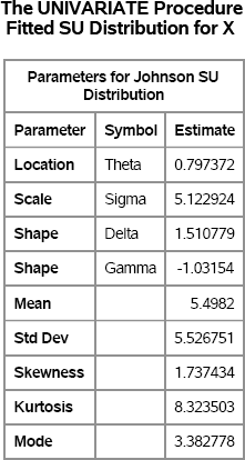
You can use PROC UNIVARIATE to verify that the simulated data are from the specified S_U distribution. Figure 7.1 shows the parameter estimates. The estimates are somewhat close to the parameters, but there appears to be substantial variability in the estimates.

   proc univariate data=SU;
      histogram x / su noplot;
      ods select ParameterEstimates;
   run;

Figure 7.1 Parameter Estimates for Simulated S_U Data

Exercise 7.3: Simulate 10,000 observations from each of the following distributions. Use PROC UNIVARIATE to verify that the parameter estimates are close to the parameter values.

1. the Gumbel distribution with μ = 1 and σ = 2
2. the inverse Gaussian distribution with μ = 1.5 and σ = 2
3. the generalized Pareto distribution with θ = 0, σ = 2, and α = –0.15
4. the power function distribution with θ = 0, σ = 2, and α = 0.15
5. the Rayleigh distribution with θ = 1 and σ = 2

Exercise 7.4: Simulate 1,000 samples, each of size 100, from the S_U distribution with θ = 1, σ = 5, δ = 1.5, and γ = – 1. Use PROC UNIVARIATE to compute the corresponding parameter estimates. (Be sure to use OPTION NONOTES for this simulation.) Draw histograms of the parameter estimates. Which estimate has the largest variance? The smallest variance? Be aware that the four-parameter estimation might not succeed for every sample.

7.4 Inverse CDF Sampling

If you know the cumulative distribution function (CDF) of a probability distribution, then you can always generate a random sample from that distribution. However, this method of sampling can be computationally expensive unless you have a formula for the inverse CDF.

This sampling technique uses the fact that a continuous CDF, F, is a one-to-one mapping of the domain of the CDF into the interval (0,1). Therefore, if U is a random uniform variable on (0, 1), then X = F^–1(U) has the distribution F. For a proof, see Ross (2006, p. 62).

7.4.1 The Inverse Transformation Algorithm

To illustrate the inverse CDF sampling technique (also called the inverse transformation algorithm), consider sampling from a standard exponential distribution. The exponential distribution has probability density f(x) = e^–x, x > 0, and therefore the cumulative distribution is This function can be explicitly inverted by setting u = F(x) and solving for x. The inverse CDF is x = F^-1 (u) = – log(1 – u).

The following DATA step generates random values from the exponential distribution by generating random uniform values from U(0,1) and applying the inverse CDF of the exponential distribution. The UNIVARIATE procedure is used to check that the data follow an exponential distribution.

/* Inverse CDF algorithm */
%let N = 100;                      /* size of sample */
data Exp(keep=x);
call streaminit(12345);
do i = 1 to &N;
   u = rand(“Uniform”);
   x = -log(1-u);
   output;
end;
run;

proc univariate data=Exp;
   histogram x / exponential(sigma=1) endpoints=0 to 6 by 0.5;
   cdfplot x / exponential(sigma=1);
   ods select GoodnessOfFit Histogram CDFPlot;
run;

Figure 7.2 Goodness-of-Fit Tests for Exponential Distribution

Figure 7.3 Histogram and Empirical CDF of Exponential Data

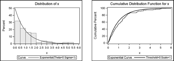
This technique is used by many statistical software packages to generate exponential random variates. Additional examples are shown in Chapter 5 of Ross (2006), which includes the current example.

Exercise 7.5: The function F(x) = x² defines a distribution on the interval [0,1]. Use the inverse function to generate 100 random values from F. Use PROC UNIVARIATE to plot the empirical CDF, which should approximate F.

7.4.2 Root Finding and the Inverse Transformation Algorithm

Even if you cannot invert the CDF, you can still use the inverse CDF algorithm by numerically solving for the quantiles of the CDF. However, because this method is computationally expensive, you should use this technique only when direct methods are not available.

If F is a distribution function, then you can simulate values from F by doing the following:

1. Generate a random uniform value u in (0,1).
2. Use bisection or some other root-finding algorithm to find the value x such that F(x) = u.
3. Repeat these steps until you have generated N values of x.

The SAS/IML 12.1 language supports the FROOT function for finding the root of a univariate function. Prior to SAS/IML 12.1, you can use the Bisection module, which is defined in Appendix A.

To illustrate this method, define the distribution function Q(x) = (x + x³ + x⁵)/3 for x on the interval [0,1]. You can test the bisection algorithm by defining the Func module to be the function Q(x) – u:

   proc iml;
   /* a quantile is a zero of the following function */
   start Func(x) global(target);
      cdf = (x + x##3 + x##5)/3;
      return( cdf-target );
   finish;
   
/* test bisection module */
target =0.5;                  /* global variable used by Func module */
/* for SAS/IML 9.3 and before, use q = Bisection(0,1); */
q = froot(“Func”, {01});     /* SAS/IML 12.1                        */

The result of the computation is a quantile of the Q distribution. If you plug the quantile into Q, then you obtain the target value. Figure 7.4 shows that the median of the quintic distribution function is approximately 0.77.

   p = (q + q##3 + q##5)/3;      /* check whether F(q) = target          */
   print q p[label=“CDF(q)”];

Figure 7.4 Median of Distribution

To simulate values from Q, generate random uniform values as target values and use the root-finding algorithm to solve for the corresponding quantiles. Figure 7.5 shows the empirical density and ECDF for 100 random observations that are drawn from Q.

   N = 100;
   call randseed(12345);
   u= j(N,1); x = j(N,1);
   call randgen(u, “Uniform”);             /* u ~ U(0,1)        */
   do i = 1 to N;
      target = u[i];
      /* for SAS/IML 9.3 and before, use x[i] = Bisection(0,1); */
      x[i] = froot(“Func”, {0 1});         /* SAS/IML 12.1      */
   end;

Figure 7.5 Histogram and Empirical CDF of Quintic Distribution

7.5 Finite Mixture Distributions

A mixture distribution is a population that contains subpopulations, which are also called components. Each subpopulation can be a different distribution, but they can also be the same distribution with different parameters. In addition to specifying the subpopulations, a mixture distribution requires that you specify mixing probabilities.

In general, a (finite) mixture distribution is composed of k components. If f_i is the PDF of the i th component, and π_i, are the mixing probabilities, then the PDF of the mixture is g(x) = where You can use the RAND function with the “Table” distribution to randomly select a subpopulation according to the mixing probabilities. For many choices of component densities, you can use the FMM procedure in SAS/STAT software to fit a finite mixture distribution to data.

7.5.1 Simulating from a Mixture Distribution

Suppose that you use a mixture distribution to model the time required to answer questions in a call center. From historic data, you subdivide calls into three types, each with its own distribution:

1. Easy questions: These questions can be answered in about three minutes. They account for about 50% of all calls. You decide to model this subpopulation by N(3,1).
2. Specialized questions: These questions require about eight minutes to answer. They account for about 30% of all calls. You decide to model this subpopulation by N(8,2).
3. Difficult questions: These questions require about 10 minutes to answer. They account for the remaining 20% of calls. You model this subpopulation by N(10, 3).

The following DATA step uses the “Table” distribution (see Section 2.4.5) to randomly select a type of question (easy, specialized, or difficult) according to historical proportions. The time required to answer each question is then modeled as a random sample from the relevant subpopulation. Figure 7.6 shows the distribution of the simulated times overlaid with a kernel density estimate (KDE).

   %let N = 100;                                  /* size of sample    */
   data Calls(drop=i);
   call streaminit(12345);
   array prob [3] _temporary_ (0.5 0.3 0.2);
   do i = 1 to &N;
      type = rand(“Table”, of prob[*]);           /* returns 1, 2, or 3 */
      if type=1 then      x = rand(“Normal”,   3, 1);
      else if type=2 then x = rand(“Normal”,   8, 2);
      else                x = rand(“Normal”,  10, 3);
      output;
   end;
   run;

   proc univariate data=Calls;
      ods select Histogram;
      histogram x / vscale=proportion
      kernel(lower=0 c=SJPI);
   run;

Figure 7.6 Sample from Mixture Distribution (N = 100)

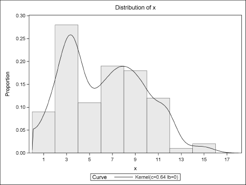
Figure 7.6 shows that the histogram and KDE have a major peak at x = 3, which corresponds to the mean of the most frequent type of question (“easy”). There is also a smaller peak at x = 8, which corresponds to the mean time for answering the “specialized” questions. The KDE also shows a small “bump” near x = 10, which corresponds to the “difficult” questions.

In order to simulate many samples, you can add an additional DO loop:

   do SampleID = 1 to &NumSamples;         /* simulation loop */
      do i = 1 to &N;
      …
      end;
   end;

From a modeling perspective, a normal distribution is probably not a good model for the “easy” questions because the N(3,1) distribution can produce negative “times.” The next exercise addresses this issue by truncating the mixture distribution at a positive value. (This is called a truncated distribution; see Section 7.7.)

Exercise 7.6: Assume that every call requires at least one minute to handle. Modify the DATA step in this section so that if x is less than 1, then it is replaced by the value 1. (This results in a mixture of a point mass and the truncated mixture distribution.) Simulate 1,000 samples from the distribution. Use PROC MEANS to compute the total time that is required to answer 100 calls. Use PROC UNIVARIATE to examine the distribution of the total times. Based on the simulation, predict how often the call center will need 11 or more hours to service 100 calls.

7.5.2 The Contaminated Normal Distribution

The contaminated normal distribution was introduced by Tukey (1960). The contaminated normal distribution is a specific instance of a two-component mixture distribution in which both components are normally distributed with a common mean. For example, a common contaminated normal model is to simulate values from an N(0,1) distribution with probability 0.9 and from an N(0,10) distribution with probability 0.1. This results in a distribution with heavier tails than normality. This is also a convenient way to generate data with outliers.

Because there are only two groups, you can use a Bernoulli random variable (instead of the more general “Table” distribution) to select the component from which each observation is drawn, as shown in the following program:

   %let std =10;                   /* magnitude of contamination */
   %let N = 100;                   /* size of sample             */
   data CN(keep=x);
   call streaminit(12345);
   do i = 1 to &N;
      if rand(“Bernoulli”, 0.1) then
         x = rand(“Normal”, 0, &std);
      else
         x = rand(“Normal”);
      output;
   end;
   run;

   proc univariate data=CN;
      var x;
      histogram x / kernel vscale=proportion endpoints=-15 to 21 by 1;
      qqplot x;
   run;

Figure 7.7 Histogram and Q-Q Plot of Contaminated Normal Sample

Johnson (1987, p. 55) states that “Many commonly used statistical methods perform abominably” with data that are generated from a contaminated normal distribution.

Exercise 7.7: It is possible to create a continuous mixture distribution by replacing a parameter with a random variable (Devroye 1986, p. 16). Simulate data from the distribution N(μ, 1), where μ ~ U(0,1). Draw a histogram of the result. The mean of the simulated data should be close to E(μ) = 1/2.

7.6 Simulating Survival Data

In medical and pharmaceutical studies, it is common to encounter time-to-event data. For example, suppose that a study contains 100 subjects. When a subject experiences the event of interest (death, remission, onset of disease,… ), the time of the event is recorded.

In the simplest situation, the event occurs at a common constant rate, which is called the hazard rate. A constant rate is equivalent to the event times being exponentially distributed. You can use the %RANDEXP macro, as described in Section 2.5.3, to generate survival times. You can analyze the survival time by using the LIFETEST procedure, as follows. The results are shown in Figure 7.8.

   /* sigma is scale parameter; use sigma=1/lambda for a rate parameter */
   %macro RandExp(sigma);
      ((&sigma) * rand(“Exponential”))
   %mend;

   data LifeData;
   call streaminit(1);
   do PatientID = 1 to 100;
      t = %RandExp(1/0.01);                /* hazard rate = 0.01 */
      output;
   end;
   run;

   proc lifetest data=LifeData;
      time t;
      ods select Quartiles Means;
   run;

Figure 7.8 Mean and Quartiles of Survival Time

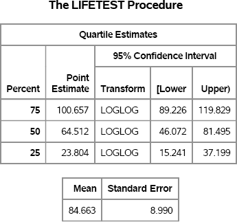
The output in Figure 7.8 shows estimates for the mean survival time and for quartiles of the survival time. For comparison, the exponential distribution with scale parameter σ has quartiles given by Q₂₅ = σ log(4/3), Q₅₀ = σ log(2), and Q₇₅ = σ log(4). The mean of the exponential distribution is σ. For σ = 100, these quartiles are approximately Q₂₅ ≈ 28.8, Q₅₀ ≈ 69.3, Q₇₅ ≈ 138.6.

The second example introduces censored observations. If a subject completes the study without experiencing the event, then the event time for that subject is said to be censored. Similarly, patients who drop out of the study prior to experiencing the event are said to be censored. Suppose that you want to simulate the following situations:

• The hazard rate for each subject is 0.01 events per day.
• The rate at which subjects drop out of the study is 0.001 per day.
• The study lasts for 365 days.

In the following DATA step, the variable Censored is an indicator variable that records whether the recorded time is the time of the event (Censored = 0) or the time of censoring (Censored = 1). The LIFETEST procedure is used to analyze the results. The output is shown in Figure 7.9 and Figure 7.10.

   data CensoredData(keep= PatientID t Censored);
   call streaminit(1);
   HazardRate = 0.01;         /* rate at which subject experiences event */
   CensorRate = 0.001;        /* rate at which subject drops out         */
   EndTime = 365;             /* end of study period                     */
   do PatientID = 1 to 100;
      tEvent = %RandExp(1/HazardRate);
      c = %RandExp(1/CensorRate);
      t = min(tEvent, c, EndTime);
      Censored = (c < tEvent | tEvent > EndTime);
      output;
   end;
   run;

   proc lifetest data=CensoredData plots=(survival(atrisk CL));
      time t*Censored(1);
      ods select Quartiles Means CensoredSummary SurvivalPlot;
   run;

Figure 7.9 Summary Statistics for Estimates of Survival Time for Censored Data

Note: The mean survival time and its standard error were underestimated because the largest observation was censored and the estimation was restricted to the largest event time.

Figure 7.10 Survival Curve for Censored Data

The analysis of censored data is sometimes called survival analysis because the event of interest is often death, but the event could also be relapse, remission, or recovery. Figure 7.10 shows the survival curve for the simulated patients. By Day 100, only 28 patients had not experienced the event. By Day 300, all but two patients had either dropped out of the study or had experienced the event.

In general, you can specify any distribution for the event times, as shown in the following exercise. See Section 12.4 for modeling survival times that include covariates.

Exercise 7.8: Simulate survival times that are lognormally distributed. For example, use exp(rand(“Normal”, 4, 1)) as the time to event. First, assume no censoring and an arbitrarily long study. Next, assume a 365-day study and a constant rate of dropping out.

7.7 The Acceptance-Rejection Technique

The rejection method is a technique for simulating values from a distribution (called the instrumental distribution) that is subject to constraints. The idea is that you generate values from the instrumental distribution and then throw away (reject) any values that do not meet the constraints. It is also known as the acceptance-rejection technique. This section explores an instructive application of the rejection method: simulating data from a truncated normal distribution (Robert 1995).

You can truncate any distribution (Devroye 1986). If X is a random variable with instrumental distribution function F, then the truncated distribution on the interval [a, b] is defined as

Here –∞ ≤ a < b ≤ ∞, with the convention that F(–∞) = 0 and F(∞) = 1.

In particular, a truncated standard normal distribution with left truncation point a has the cumulative distribution function (Φ(x)) – Φ(a))/(1 – Φ(a)), where Φ is the standard normal distribution function.

The obvious simulation algorithm for a truncated normal random variable is to simulate from a normal distribution and discard any value outside of the interval [a, b]. For example, the following DATA step simulates data from the truncated normal distribution with left truncation point a = 0:

   %let N = 100;                         /* size of sample */
   data TruncNormal(keep=x);
   call streaminit(12345);
   a = 0;
   do i = 1 to &N;
      do until( x>=a );                   /* reject x < a */
         x = rand(“Normal”);
      end;
      output;
   end;
   run;

In a similar manner, you can simulate from a doubly truncated normal distribution on the interval [0,2]:

   do until( (x>0 & x<2) );          /* x in (0, 2) */
      x = rand(“Normal”);
   end;

This technique is appropriate when the truncation points are near the middle of the normal distribution. For truncation points that are in the tails of the normal distribution, see the accept-reject algorithm in Robert (1995). See also Devroye (1986, p. 380).

An alternative approach to the rejection technique is to use the inverse CDF technique. This technique is applicable for any truncated distribution G, but requires computing the inverse CDF, which can be expensive. To implement this technique, first generate U ~ U(0,1). Then the random variable Y = G ^–1(U) = F ^–1(F(a) + U(F(b) – F(a))) is distributed according to G. For the left-truncated standard normal distribution, use the following SAS statements:

   Phi_a = cdf(“Normal”, 0);              /* a = 0        */
   Phi_b =1;                              /* b = infinity */
   do i = 1 to &N;
      u = rand(“Uniform”);
      x = quantile(“Normal”, Phi_a + u*(Phi_b - Phi_a));
      output;
   end;

For implementing univariate accept-reject techniques, the DATA step has an advantage over the SAS/IML language. It can be a challenge to implement time-to-event and accept-reject algorithms in the SAS/IML language because you do not know ahead of time how many random values to simulate. An effective technique is to multiply the number of observations that you want by some large factor. For example, for the truncated normal distribution with a truncation point of zero, you can expect half of the random normal variates to be rejected. To be on the safe side, simulate more than twice as many normal variates as you need for the truncated normal distribution as shown in the following SAS/IML program:

   proc iml;
   call randseed(12345);
   multiple = 2.5;                /* choose value > 2                */
   y = j(multiple * &N, 1);       /* allocate more than you need    */
   call randgen(y, “Normal”);     /* y ~ N(0,1)                     */
   idx = loc(y > 0);              /* acceptance step                */
   x = y[idx];
   x = x[1:&N];                   /* discard any extra observations */

A more statistical approach is to use the QUANTILE function to estimate the proportion of simulated data that are likely to be rejected during the simulation. You then sample enough variates from the instrumental distribution to be 99.9% certain that you will obtain at least N observations from the truncated distribution.

For the truncated normal distribution, p = 0.5 is the probability that a variate from the instrumental distribution is accepted. The event “accept the instrumental variate” is a Bernoulli random variable with probability of success p. The negative binomial is the distribution of the number of failures before N successes in a sequence of independent Bernoulli trials. You can compute F, the 99.9th percentile of the number of failures that you encounter before you obtain N successes. Therefore, the total number of trials that you need is M = F + N.

For the truncate normal distribution, the following SAS/IML statements compute these quantities. The computation indicates that you should generate 248 normal variates in order to be 99.9% certain that you will obtain at least 100 variates for the truncated normal distribution. See Figure 7.11.

   p = 0.5;             /* prob of accepting instrumental variate */
   F = quantile(“NegBin”, 0.999, p, &N);
   M = F + &N;          /* Num Trials = failures + successes      */
   print M;

Figure 7.11 Number of Trials to Generate N = 100 Variates

Exercise 7.9: Create a histogram for the truncated normal distributions in this section.

Exercise 7.10: Generate 10,000 samples of size 248 from the normal distribution and discard any negative observations to obtain a truncated normal sample. The size of the truncated normal sample varies. Plot a histogram of the sample sizes. How many samples have fewer than 100 observations?

7.8 References

Bowman, K. O. and Shenton, L. R. (1983), “Johnson's System of Distributions,” in S. Kotz, N. L. Johnson, and C. B. Read, eds., Encyclopedia of Statistical Sciences, volume 4, 303–314, New York: John Wiley & Sons.

Devroye, L. (1986), Non-uniform Random Variate Generation, New York: Springer-Verlag. URL http://luc.devroye.org/rnbookindex.html

Johnson, M. E. (1987), Multivariate Statistical Simulation, New York: John Wiley & Sons.

Johnson, N. L. (1949), “Systems of Frequency Curves Generated by Methods of Translation,” Biometrika, 36, 149–176.

Johnson, N. L., Kotz, S., and Balakrishnan, N. (1994), Continuous Univariate Distributions, volume 1, 2nd Edition, New York: John Wiley & Sons.

Robert, C. P. (1995), “Simulation of Truncated Normal Variables,” Statistics and Computing, 5, 121–125.

Ross, S. M. (2006), Simulation, 4th Edition, Orlando, FL: Academic Press.

Tukey, J. W. (1960), “A Survey of Sampling from Contaminated Distributions,” in I. Olkin, ed., Contributions to Probability and Statistics, Stanford, CA: Stanford University Press.