
Chapter 2
Simulating Data from Common Univariate Distributions
Contents
2.1 Introduction to Simulating Univariate Data
2.2 Getting Started: Simulate Data from the Standard Normal Distribution
2.3 Template for Simulating Univariate Data in the DATA Step
2.4 Simulating Data from Discrete Distributions
2.4.1 The Bernoulli Distribution
2.4.2 The Binomial Distribution
2.4.3 The Geometric Distribution
2.4.4 The Discrete Uniform Distribution
2.4.6 The Poisson Distribution
2.5 Simulating Data from Continuous Distributions
2.5.2 The Uniform Distribution
2.5.3 The Exponential Distribution
2.6 Simulating Univariate Data in SAS/IML Software
2.6.1 Simulating Discrete Data
2.6.2 Sampling from Finite Sets
2.6.3 Simulating Continuous Data
2.1 Introduction to Simulating Univariate Data
There are three primary ways to simulate data in SAS software:
- Use the DATA step to simulate data from univariate and uncorrelated multivariate distributions. You can use the RAND function to generate random values from more than 20 standard univariate distributions. You can combine these elementary distributions to build more complicated distributions.
- Use the SAS/IML language to simulate data from many distributions, including correlated multivariate distributions. You can use the RANDGEN subroutine to generate random values from standard univariate distributions, or you can use several predefined modules to generate data from multivariate distributions. You can extend the SAS/IML language by defining new functions that sample from distributions that are not built into SAS.
- Use specialized procedures in SAS/STAT software and SAS/ETS software to simulate data with special properties. Procedures that generate random samples include the SIMNORMAL, SIM2D, and COPULA procedures.
This chapter describes the two most important techniques that are used to simulate data in SAS software: the DATA step and the SAS/IML language. Although the DATA step is a useful tool for simulating univariate data, SAS/IML software is more powerful for simulating multivariate data. To learn how to use the SAS/IML language effectively, see Wicklin (2010).
Most of the terminology in this book is standard. However, a term that you might not be familiar with is the term random variate. A random variate is a particular outcome of a random variable (Devroye 1986). For example, let X be a Bernoulli random variable that takes on the value 1 with probability p and the value 0 with probability 1 – p. If you draw five observations from the probability distribution, you might obtain the values 0, 1, 1, 0, 1. Those five numbers are random variates. This book also uses the terms “simulated values” and “simulated data.” Some authors refer to simulated data as “fake data.”
2.2 Getting Started: Simulate Data from the Standard Normal Distribution
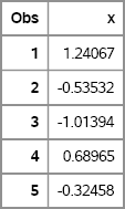
To “simulate data” means to generate a random sample from a distribution with known properties. Because an example is often an effective way to convey main ideas, the following DATA step generates a random sample of 100 observations from the standard normal distribution. Figure 2.1 shows the first five observations.
data Normal(keep=x);
call streaminit(4321);                /* Step 1 */
do i = 1 to 100;                      /* Step 2 */
   x = rand(“Normal”);                /* Step 3 */
   output;
end;
run;

proc print data=Normal(obs=5);
run;
Figure 2.1 A Few Observations from a Normal Distribution
The DATA step consists of three steps:
- Set the seed value with the STREAMINIT function. Seeds for random number generation are discussed further in Section 3.3.
- Use a DO loop to iterate 100 times.
- For each iteration, call the RAND function to generate a random value from the standard normal distribution.
If you change the seed value, you will get a different random sample. If you change the number 100, you will get a sample with a different number of observations. To get a nonnormal distribution, change the name of the distribution from “Normal” to one of the families listed in Section 2.7. Some distributions, including the normal distribution, include parameters that you can specify after the name.
2.3 Template for Simulating Univariate Data in the DATA Step
It is easy to generalize the example in the previous section. The following SAS pseudocode shows a basic template that you can use to generate N observations with a specified distribution:
%let N = 100;             /* size of sample                     */

data Sample(keep=x);
call streaminit(4321);    /* or use a different seed            */
do i = 1 to &N;           /* &N is the value of the N macro var */
   /* specify distribution and parameters */
   x = rand(“DistribName”, param1, param2, …);
   output;
end;
run;
The simulated data are written to the Sample data set. The macro variable N is defined in order to emphasize the role of that parameter. The expression &N is replaced by the value of the macro parameter (here, 100) before the DATA step is run.
The (pseudo) DATA step demonstrates the following steps for simulating data:
- A call to the STREAMINIT subroutine, which specifies the seed that initializes the random number stream. When the argument is a positive integer, as in this example, the random sequence is reproducible. If you specify 0 as the argument, the random number sequence is initialized from your computer's internal system clock. This implies that the random sequence will be different each time that you run the program. Seeds for random number generation are discussed in Section 3.3.
- A DO loop that iterates N times.
- A call to the RAND function, which generates one random value each time that the function is called. The first argument is the name of a distribution. The supported distributions are enumerated in Section 2.7. Subsequent arguments are parameter values for the distribution.
2.4 Simulating Data from Discrete Distributions
When the set of possible outcomes is finite or countably infinite (like the integers), assigning a probability to each outcome creates a discrete probability distribution. Of course, the sum of the probabilities over all outcomes is unity.
The following sections generate a sample of size N = 100 from some well-known discrete distributions. The code is followed by a frequency plot of the sample, which is overlaid with the exact probabilities of obtaining each value. You can use PROC FREQ to compute the empirical distribution of the data; the exact probabilities are obtained from the probability mass function (PMF) of the distribution. Section 3.4.2 describes how to overlay a bar chart with a scatter plot that shows the theoretical probabilities.
2.4.1 The Bernoulli Distribution
The Bernoulli distribution is a discrete probability distribution on the values 0 and 1. The probability that a Bernoulli random variable will be 1 is given by a parameter, p, 0 ≤ p ≤ 1. Often a 1 is labeled a “success,” whereas a 0, which occurs with probability 1 – p, is labeled a “failure.”
The following DATA step generates a random sample from the Bernoulli distribution with p = 1/2. If you identify x = 1 with “heads” and x = 0 with “tails,” then this DATA step simulates N = 100 tosses of a fair coin.
%let N = 100;
data Bernoulli(keep=x);
call streaminit(4321);
p = 1/2;
do i = 1 to &N;
   x = rand(“Bernoulli”, p);         /* coin toss */
   output;
end;
run;
You can use the FREQ procedure to count the outcomes in this simulated data. For this sample, the value 0 appeared 52 times, and the value 1 appeared 48 times. These frequencies are shown by the bar chart in Figure 2.2. The expected percentages for each result are shown by the round markers.
Figure 2.2 Sample from Bernoulli Distribution (p = 1/2) Overlaid with PMF

If X is a random variable from the Bernoulli distribution, then the expected value of X is p and the variance is p(1 – p). In practice, this means that if you generate a large random sample from the Bernoulli distribution, you can expect the sample to have a sample mean that is close to p and a sample variance that is close to p(1 – p).
2.4.2 The Binomial Distribution
Imagine repeating a Bernoulli trial n times, where each trial has a probability of success equal to p. If p is large (near 1), you expect most of the Bernoulli trials to be successes and only a few of the trials to be failures. On the other hand, if p is near 1/2, you expect to get about n/2 successes.
The binomial distribution models the number of successes in a sequence of n independent Bernoulli trials. The following DATA step generates a random sample from the binomial distribution with p = 1/2 and n = 10. This DATA step simulates a series of coin tosses. For each trial, the coin is tossed 10 times and the number of heads is recorded. This experiment is repeated N = 100 times. Figure 2.3 shows a frequency plot of the results.
data Binomial(keep=x);
call streaminit(4321);
p = 1/2;
do i = 1 to &N;
   x = rand(“Binomial”, p, 10);    /* number of heads in 10 tosses */
   output;
end;
run;
Figure 2.3 Sample from Binomial Distribution (p = 1/2, n = 10) Overlaid with PMF

For this series of experiments, you expect to get five heads most frequently, followed closely by four and six heads. The expected percentages are indicated by the round markers. For this particular simulation, Figure 2.3 shows that four heads and six heads appeared more often than five heads appeared. The sample values are shown by the bars; the expected percentages are shown by round markers.
If X is a random variable from the binomial(p, n) distribution, then the expected value of X is np and the variance is np(1 – p). In practice, this means that if you generate a large random sample from the binomial(p, n) distribution, then you can expect the sample to have a sample mean that is close to np.
Some readers might be concerned that the distribution of the sample shown in Figure 2.3 differs so much from the theoretical distribution of the binomial distribution. This deviation is not an indication that something is wrong. Rather, it demonstrates sampling variation. When you simulate data from a population model, the data will almost always look slightly different from the distribution of the population. Some values will occur more often than expected; some will occur less often than expected. This is especially apparent in small samples and for distributions with large variance. It is this sampling variation that makes simulation so valuable.
2.4.3 The Geometric Distribution
How many times do you need to toss a fair coin before you see heads? Half the time you will see heads on the first toss, one quarter of the time it requires two tosses, and so on. This is an example of a geometric distribution.
In general, the geometric distribution models the number of Bernoulli trials (with success probability p) that are required to obtain one success. An alternative definition, which is used by the MCMC procedure in SAS, is to define the geometric distribution to be the number of failures before the first success.
You can simulate a series of coin tosses in which the coin is tossed until a heads appears and the number of tosses is recorded. If p is the probability of tossing heads, then the following statement generates an observation from the Geometric(p) distribution:
x = rand(“Geometric”, p); /* number of trials until success */
Figure 3.6 shows a graph of simulated geometric data and an overlaid PMF.
If X is a random variable from the geometric(p) distribution, then the expected value of X is 1/p and the variance is (1 – p)/p2.
Exercise 2.1: Write a DATA step that simulates observations from a Geometric(0.5) distribution.
2.4.4 The Discrete Uniform Distribution
A Bernoulli distribution models two outcomes. You can model situations in which there are multiple outcomes by using either the discrete uniform distribution or the “Table” distribution (see the next section).
When you toss a standard six-sided die, there is an equal probability of seeing any of the six faces. You can use the discrete uniform distribution to produce k integers in the range [1, k]. SAS does not have a built-in discrete uniform distribution. Instead, you can use the continuous uniform distribution to produce a random number u in the interval (0, 1), and you can use the CEIL function to produce the smallest integer that is greater than or equal to ku.
The following DATA step generates a random sample from the discrete uniform distribution with k = 6. This DATA step simulates N = 100 rolls of a fair six-sided die.
data Uniform(keep=x);
call streaminit(4321);
k = 6;                              /* a six-sided die         */
do i = 1 to &N;
   x = ceil(k * rand(“Uniform”));   /* roll 1 die with k sides */
   output;
end;
run;
You can also simulate data with uniform probability by using the “Table” distribution, which is described in the next section.
To check the empirical distribution of the simulated data, you can use PROC FREQ to show the distribution of the x variable. The results are shown in Figure 2.4. As expected, each number 1,2,…,6 is generated about 16% of the time.
proc freq data=Uniform;
   tables x / nocum;
run;
Figure 2.4 Sample from Uniform Distribution (k = 6)

2.4.5 Tabulated Distributions
In some situations there are multiple outcomes, but the probabilities of the outcomes are not equal. For example, suppose that there are 10 socks in a drawer: five are black, two are brown, and three are white. If you close your eyes and draw a sock at random, the probability of that sock being black is 0.5, the probability of that sock being brown is 0.2, and the probability of that sock being white is 0.3. After you record the color of the sock, you can replace the sock, mix up the drawer, close your eyes, and draw again.
The RAND function supports a “Table” distribution that enables you to specify a table of probabilities for each of k outcomes. You can use the “Table” distribution to sample with replacement from a finite set of outcomes where you specify the probability for each outcome. In SAS/IML software, you can use the RANDGEN or SAMPLE routines.
The following DATA step generates a random sample of size N = 100 from the “Table” distribution with probabilities p = {0.5, 0.3, 0.2}. You can use PROC FREQ to display the observed frequencies, which are shown in Figure 2.5.
data Table(keep=x);
call streaminit(4321);
p1 = 0.5; p2 = 0.2; p3 = 0.3;
do i = 1 to &N;
   x = rand(“Table”, p1, p2, p3);      /* sample with replacement */
   output;
end;
run;

proc freq data=Table;
   tables x / nocum;
run;
Figure 2.5 Sample from “Table” Distribution (p = {0.5, 0.2, 0.3})

For the simulated sock experiment with the given probabilities, a black sock (category 1) was drawn 48 times, a brown sock (category 2) was drawn 21 times, and a white sock was drawn 31 times.
If you have many potential outcomes, it would be tedious to specify the probabilities of each outcome by using a comma-separated list. Instead, it is more convenient to specify an array in the DATA step to hold the probabilities, and to use the OF operator to list the values of the array as shown in the following example:
data Table(keep=x);
call streaminit(4321);
array p[3] _temporary_ (0.5 0.2 0.3);
do i = 1 to &N;
   x = rand(“Table”, of p[*]);             /* sample with replacement */
   output;
end;
run;
The _TEMPORARY_ keyword makes p a temporary array that holds the parameter values. The elements of a temporary array do not have names and are not written to the output data set, which means that you do not need to use a DROP or KEEP option to omit them from the data set.
The “Table” distribution is related to the multinomial distribution, which is discussed in Section 8.2. If you generate N observations from the “Table” distribution and tabulate the frequencies for each category, then the frequency vector is a single observation from the multinomial distribution. Consequently, the “Table” and multinomial distributions are related in the same way that the Bernoulli and binomial distributions are related.
Exercise 2.2: Use the “Table” distribution to simulate rolls from a six-sided die.
2.4.6 The Poisson Distribution
Suppose that during the work day a worker receives email at an average rate of four messages per hour. What is the probability that she might get seven messages in an hour? Or that she might get only one message? The Poisson distribution models the counts of an event during a given time period, assuming that the event happens at a constant average rate.
For an average rate of λ events per time period, the expected value of a random variable from the Poisson distribution is λ, and the variance is also λ.
The following DATA step generates a random sample from the Poisson distribution with λ = 4. This DATA step simulates the number of emails that a worker receives each hour, under the assumption that the number of emails arrive at a constant average rate of four emails per hour. This experiment simulates N = 100 hours at work. The results are shown in Figure 2.6.
data Poisson(keep=x);
call streaminit(4321);
lambda = 4;
do i = 1 to &N;
   x = rand(“Poisson”, lambda);               /* num events per unit time */
   output;
end;
run;
Figure 2.6 Sample from Poisson Distribution (λ = 4) Overlaid with PMF

For the Poisson model, the worker can expect to receive four emails during a one-hour period about 20% of the time. The same is true for receiving three emails in an hour. She can expect to receive six emails during an hour slightly more than 10% of the time. These expected percentages are shown by the round markers. The “actual” number of emails received during each hour is shown by the bar chart for the 100 simulated hours. There were 18 one-hour periods during which the worker received three emails. There were 11 one-hour periods during which the worker received six emails.
Exercise 2.3: A negative binomial variable is defined as the number of failures before k successes in a series of independent Bernoulli trials with probability of success p. Define a trial as rolling a six-sided die until a specified face appears k = 3 times. Simulate 1,000 trials and plot the distribution of the number of failures.
2.5 Simulating Data from Continuous Distributions
When the set of possible outcomes is uncountably infinite (like an interval or the set of real numbers), assigning a probability to each outcome creates a continuous probability distribution. Of course, the integral of the probabilities over the set is unity.
The following sections generate a sample of size N = 100 from some well-known continuous distributions. Most sections also show a histogram of the sample that is overlaid with the probability density curve for the population. The probability density function (PDF) is described in Section 3.2. Section 3.4.3 describes how to create the graphs.
See Table 2.3 for a list of common distributions that SAS supports.
2.5.1 The Normal Distribution
The normal distribution with mean μ and standard deviation σ is denoted by N(μ, σ). Its density is given by the following:
![]()
The standard normal distribution sets μ = 0 and σ = 1.
Many physical quantities are modeled by the normal distribution. Perhaps more importantly, the sampling distribution of many statistics are approximately normally distributed.
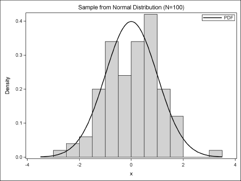
Section 2.2 generated 100 observations from the standard normal distribution. Figure 2.7 shows a histogram of the simulated data along with the graph of the probability density function. For this sample, the histogram bars are below the PDF curve for some intervals and are greater than the curve for other intervals. A second sample of 100 observations is likely to produce a different histogram.
Figure 2.7 Sample from a Normal Distribution (μ = 0, σ = 1) Overlaid with PDF
To explicitly specify values of the location and scale parameters, define mu and sigma outside of the DO loop, and then use the following statement inside the DO loop:
x = rand(“Normal”, mu, sigma); /* × ~ N(mu, sigma) */
If X is a random variable from the N(μ, σ) distribution, then the expected value of X is μ and the variance is σ2. Be aware that some authors denote the normal distribution by N(μ, σ2), where the second parameter indicates the variance. This book uses N(μ, σ) instead, which matches the meaning of the parameters in the RAND function.
2.5.2 The Uniform Distribution
The uniform distribution is one of the most useful distributions in statistical simulation. One reason is that you can use the uniform distribution to sample from a finite set. Another reason is that “random variates with various distributions can be obtained by cleverly manipulating” independent, identically distributed uniform variates (Devroye 1986, p. 206).
The uniform distribution on the interval (a, b) is denoted by U(a, b). Its density is given by f (x) = (b – a)–1 for x in (a, b). The standardized uniform distribution on [0, 1] (often called the uniform distribution) is denoted U(0, 1).
You can use the following statement in the DATA step to generate a random observation from the standard uniform distribution:
x = rand(“Uniform”); /* X ~ U(0, 1) */
The uniform random number generator never generates the number 0 nor the number 1. Therefore, all values are in the open interval (0, 1).
You can also use the uniform distribution to sample random values from U(a, b). To do this, define a and b outside of the DO loop, and then use the following statement inside the DO loop:
y = a + (b-a)*rand(“Uniform”); /* Y ~ U(a, b) */
If X is a random variable from the standard uniform distribution, then the expected value of X is 1/2 and the variance is 1/12. In general, the uniform distribution on (a, b) has a uniform density of 1/(b – a). If Y is a random variable from the U(a, b), the expected value of Y is (a + b)/2 and the variance is (b – a)2/12.
Exercise 2.4: Generate 100 observations from a uniform distribution on the interval (–1, 1).
2.5.3 The Exponential Distribution
The exponential distribution models the time between events that occur at a constant average rate. The exponential distribution is a continuous analog of the geometric distribution. The classic usage of the exponential distribution is to model the time between detecting particles emitted during radioactive decay.
The exponential distribution with scale parameter σ is denoted Exp(σ). Its density is given by f (x) = (1/σ) exp(–x/σ) for x > 0. Alternatively, you can use λ = 1/σ, which is called the rate parameter. The rate parameter describes the rate at which an event occurs.
The following DATA step generates a random sample from the exponential distribution with scale parameter σ = 10. A histogram of the sample is shown in Figure 2.8.
data Exponential(keep=x);
call streaminit(4321);
sigma = 10;
do i = 1 to &N;
   x = sigma * rand(“Exponential”);      /* X ~ Expo(10) */
   output;
end;
run;
Figure 2.8 Sample from the Exponential Distribution (σ = 10) Overlaid with PDF

Notice that the scale parameter for the exponential distribution is not supported by the RAND function as of SAS 9.3. However, you can show that if X is distributed according to an exponential distribution with unit scale parameter, then Y = σX is distributed exponentially with scale parameter σ. The expected value of X is σ; the variance is σ2. For example, the data shown in Figure 2.8 have a mean close to σ = 10.
If you use the exponential distribution with a scale parameter frequently, you might want to define and use the following SAS macro, which is used in Chapter 7 and in Chapter 12:
%macro RandExp(sigma);
   ((&sigma) * rand(“Exponential”))
%mend;
The following statement shows how to call the macro from the DATA step:
x = %RandExp(sigma);
Exercise 2.5: Some distributions include the exponential distribution for particular values of the distribution parameters. For example, a Weibull(1, b) distribution is an exponential distribution with scale parameter b. Modify the program in this section to simulate data as follows:
x = rand(“Weibull”, 1, sigma);
Do you obtain a similar distribution of values? Use PROC UNIVARIATE to fit the exponential model to the simulated data.
2.6 Simulating Univariate Data in SAS/IML Software
You can also generate random samples by using the RANDGEN subroutine in SAS/IML software. The RANDGEN subroutine uses the same algorithms as the RAND function, but it fills an entire matrix at once, which means that you do not need a DO loop.
The following SAS/IML pseudocode simulates N observations from a named distribution:
%let N = 100;
proc iml;
call randseed(4321);                              /* or use a different seed */
x = j(1, &N);                                   /* allocate vector or matrix */
call randgen(x, “DistribName param1”, param2,…);                   /* fill x */
The PROC IML program contains the following function calls:
- A call to the RANDSEED subroutine, which specifies the seed that initializes the random number stream. If the argument is a positive integer, then the sequence is reproducible. Otherwise, the system time is used to initialize the random number stream, and the sequence will be different each time that you run the program.
- A call to the J function, which allocates a matrix of a certain size. The syntax
J(r, c)creates an r × c matrix. For this example,xis a vector that has one row andNcolumns. - A call to the RANDGEN subroutine, which fills the elements of
xwith random values from a named distribution. The supported distributions are listed in Section 2.7.
When you use the J function to allocate a SAS/IML matrix, the matrix is filled with 1s by default. However, you can use an optional third argument to fill the matrix with another value. For example y=j(1, 5,0) allocates a 1 × 5 vector where each element has the value 0, and y=j(4, 3,.) allocates a 4 × 3 matrix where each element is a SAS missing value.
Notice that the SAS/IML implementation is more compact than the DATA step implementation. It does not create a SAS data set, but instead holds the simulated data in memory in the x vector. By not writing a data set, the SAS/IML program is more efficient. However, both programs are blazingly fast. On the author's PC, generating a million observations with the DATA step takes about 0.2 seconds. Simulating the same data in PROC IML takes about 0.04 seconds.
2.6.1 Simulating Discrete Data
The RANDGEN subroutine in SAS/IML software supports the same distributions as the RAND function. Because the IML procedure does not need to create a data set that contains the simulated data, well-written simulations in the SAS/IML language have good performance characteristics.
The previous sections showed how to use the DATA step to generate random data from various distributions. The following SAS/IML program generates samples of size N = 100 from the same set of distributions:
proc iml;
/* define parameters */
p = 1/2; lambda =4; k = 6;  prob = {0.5 0.2 0.3};

/* allocate vectors */
N = 100;
Bern = j(1, N);   Bino = j(1, N);    Geom = j(1, N);
Pois = j(1, N);   Unif = j(1, N);    Tabl = j(1, N);

/* fill vectors with random values */
call randseed(4321);
call randgen(Bern, “Bernoulli”, p);      /* coin toss                */
call randgen(Bino, “Binomial”, p, 10);   /* num heads in 10 tosses   */
call randgen(Geom, “Geometric”, p);      /* num trials until success */
call randgen(Pois, “Poisson”, lambda);   /* num events per unit time */
call randgen(Unif, “Uniform”);           /* uniform in (0, 1)        */
Unif = ceil(k * Unif);                   /* roll die with k sides    */
call randgen(Tabl, “Table”, prob);       /* sample with replacement  */
Notice that in the SAS/IML language, which supports vectors in a natural way, the syntax for the “Table” distribution is simpler than in the DATA step. You simply define a vector of parameters and pass the vector to the RANDGEN subroutine. For example, you can use the following SAS/IML program to simulate data from a discrete uniform distribution as described in Section 2.4.4. The program simulates the roll of a six-sided die by using the RANDGEN subroutine to sample from six outcomes with equal probability:
proc iml;
call randseed(4321);
prob = j(6, 1, 1)/6;               /* equal prob. for six outcomes */
d = j(1, &N);                      /* allocate 1 × N vector        */
call randgen(d, “Table”, prob);    /* fill with integers in 1–6    */
2.6.2 Sampling from Finite Sets
It can be useful to sample from a finite set of values. The SAS/IML language provides three functions that you can use to sample from finite sets:
- The RANPERM function generates random permutations of a set with n elements. Use this function to sample without replacement from a finite set with equal probability of selecting any item.
- The RANPERK function (introduced in SAS/IML 12.1) generates random permutations of k items that are chosen from a set with n elements. Use this function to sample k items without replacement from a finite set with equal probability of selecting any item.
- The SAMPLE function (introduced in SAS/IML 12.1)generates a random sample from a finite set. Use this function to sample with replacement or without replacement. This function can sample with equal probability or with unequal probability.
Each of these functions uses the same random number stream that is set by the RANDSEED routine. DATA step versions of the RANPERM and RANPERK functions are also supported.
These functions are similar to the “Table” distribution in that you can specify the probability of sampling each element in a finite set. However, the “Table” distribution only supports sampling with replacement, whereas these functions are suitable for sampling without replacement.
As an example, suppose that you have 10 socks in a drawer as in Section 2.4.5. Five socks are black, two socks are brown, and three socks are white. The following SAS/IML statements simulate three possible draws, without replacement, of five socks. The results are shown in Figure 2.9.
proc iml;
call randseed(4321);
socks = {“Black” “Black” “Black” “Black” “Black”
         “Brown” “Brown” “White” “White” “White”};
params = { 5,                         /* sample size                */
           3 };                       /* number of samples          */
s = sample(socks, params, “WOR”);     /* sample without replacement */
print s;
Figure 2.9 Random Sample without Replacement

The SAMPLE function returns a 3 × 5 matrix, s. Each row of s is an independent draw of five socks (because param[1] = 5). After each draw, the socks are returned to the drawer and mixed well. The experiment is repeated three times (because param[2] = 3). Because each draw is without replacement, no row can have more than two brown socks or more than three white socks.
2.6.3 Simulating Continuous Data
Section 2.6.1 shows how to simulate data from discrete distributions in SAS/IML software. In the same way, you can simulate data from continuous distributions by calling the RANDGEN subroutine. As before, if you allocate a vector or matrix, then a single call of the RANDGEN subroutine fills the entire matrix with random values.
The following SAS/IML program generates samples of size N = 100 from the normal, uniform, and exponential distributions:
proc iml;
/* define parameters */
mu = 3; sigma = 2;

/* allocate vectors */
N = 100;
StdNor = j(1, N);  Normal = j(1, N);
Unif = j(1, N);    Expo   = j(1, N);
/* fill vectors with random values */
call randseed(4321);
call randgen(StdNor, “Normal”);                /* N(0, 1)      */
call randgen(Normal, “Normal”, mu, sigma);     /* N(mu, sigma) */
call randgen(Unif, “Uniform”);                 /* U(0, 1)      */
call randgen(Expo, “Exponential”);             /* Exp(1)      */
2.7 Univariate Distributions Supported in SAS Software
In SAS software, the RAND function in Base SAS software and the RANDGEN subroutine in SAS/IML software are the main tools for simulating data from “named” distributions. These two functions call the same underlying numerical routines for computing random variates. However, there are some differences, as shown in Table 2.1:
Table 2.1 Differences Between RAND and RANDGEN Functions
| RAND Function | RANDGEN Subroutine | |
| Called from: | DATA step | PROC IML |
| Seed set by: | CALL STREAMINT | CALL RANDSEED |
| Returns: | Scalar value | Vector or matrix of values |
Because SAS/IML software can call Base SAS functions, it is possible to call the RAND function from a SAS/IML program. However, this is rarely done because it is more efficient to use the RANDGEN subroutine to generate many random variates with a single call.
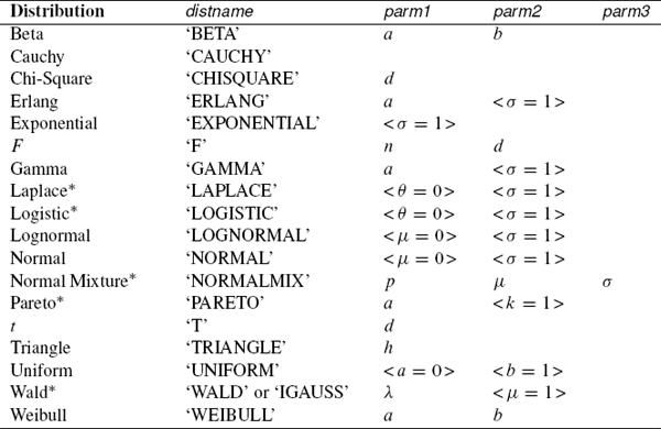
Table 2.2 and Table 2.3 list the discrete and continuous distributions that are built into SAS software. Except for the t, F, and “NormalMix” distributions, you can identify a distribution by its first four letters. Parameters for each distribution are listed after the distribution name. Parameters in angled brackets are optional. If an optional parameter is omitted, then the default value is used.
The functions marked with an asterisk are supported by the RANDGEN function in SAS/IML 12.1. In general, parameters named μ and θ are location parameters, whereas σ denotes a scale parameter.
Table 2.2 Parameters for Discrete Distributions

Table 2.3 Parameters for Continuous Distributions
Densities for all supported distributions are included in the documentation for the RAND function in SAS Functions and CALL Routines: Reference.
2.8 References
Devroye, L. (1986), Non-uniform Random Variate Generation, New York: Springer-Verlag. URL http://luc.devroye.org/rnbookindex.html
Wicklin, R. (2010), Statistical Programming with SAS/IML Software, Cary, NC: SAS Institute Inc.