
Chapter 5
Using Simulation to Evaluate Statistical Techniques
Contents
5.1 Overview of Evaluating Statistical Techniques
5.2 Confidence Interval for a Mean
5.2.1 Coverage for Normal Data
5.2.2 Coverage for Nonnormal Data
5.2.3 Computing Coverage in the SAS/IML Language
5.3 Assessing the Two-Sample t Test for Equality of Means
5.3.1 Robustness of the t Test to Unequal Variances
5.3.2 Robustness of the t Test to Nonnormal Populations
5.3.3 Assessing the t Test in SAS/IML Software
5.3.4 Summary of the t Test Simulations
5.4 Evaluating the Power of the t Test
5.4.2 A Simulated Power Analysis
5.5 Effect of Sample Size on the Power of the t Test
5.1 Overview of Evaluating Statistical Techniques
This chapter describes how to use simulation to evaluate the performance of statistical techniques. The main idea is to use the techniques from Chapter 4, “Simulating Data to Estimate Sampling Distributions,” to simulate many sets of data from a known distribution and to analyze the corresponding sampling distribution for a statistic. If you change the distribution of the population, then you also change the sampling distribution.
This chapter examines sampling distributions for several well-known statistics. For some statistics, the sampling distribution is only known asymptotically for large samples. This chapter applies simulation techniques to approximate the sampling distributions of these familiar statistics. The value of this chapter is that you can apply the same techniques to statistics for which the sampling distribution is unknown and to small samples where the asymptotic formulas do not apply. Often, simulation is the only technique for estimating the sampling distribution of an unfamiliar statistic.
This chapter describes how to use simulation to do the following:
- Estimate the coverage probability for the confidence interval for the mean of normal data. How does the coverage probability change when the data are nonnormal?
- Examine the performance of the standard two-sample t test. How does the test perform on data that do not satisfy the assumptions of the test?
- Estimate the power of the two-sample t test.
5.2 Confidence Interval for a Mean
A confidence interval is an interval estimate that contains the parameter with a certain probability. Each sample results in a different confidence interval. Due to sampling variation, the confidence interval that is constructed from a particular sample might not contain the parameter.
A 95% confidence interval is a statement about the probability that a confidence interval contains the parameter. In practical terms, a 95% confidence interval means that if you generate a large number of samples and construct the corresponding confidence intervals, then about 95% of the intervals will contain the parameter.
5.2.1 Coverage for Normal Data
You can use simulation to estimate the coverage probability of a confidence interval. Suppose you sample from the normal distribution. Let ![]() be the sample mean and s be the sample standard deviation. The exact 95% confidence interval for the population mean is
be the sample mean and s be the sample standard deviation. The exact 95% confidence interval for the population mean is
![]()
where t1−α/2, n−1 is the (1 − α/2) quantile of the t distribution with n − 1 degrees of freedom (Ross 2006, p. 118). This computation is available in the MEANS procedure by using the LCLM= option and UCLM= option in the OUTPUT statement.
This section uses simulation of normal data to demonstrate that the coverage probability of the confidence interval is 0.95. A subsequent section violates the assumption of normality and explores what happens to the coverage probability if you use these intervals with nonnormal data.
The following DATA step generates 10,000 samples, each of size 50, from the standard normal distribution. The MEANS procedure computes the mean and 95% confidence interval for each sample. These sample statistics are stored in the OutStats data set.
%let N = 50;                                  /* size of each sample  */
%let NumSamples = 10000;                      /* number of samples    */
/* 1. Simulate obs from N(0,1) */
data Normal(keep=SampleID x);
call streaminit(123);
do SampleID = 1 to &NumSamples;               /* simulation loop      */
   do i = 1 to &N;                            /* N obs in each sample */
      x = rand(“Normal”);                     /* x ~ N(0,1)           */
      output;

   end;
end;
run;

/* 2. Compute statistics for each sample */
proc means data=Normal noprint;
   by SampleID;
   var x;
   output out=OutStats mean=SampleMean lclm=Lower uclm=Upper;
run;
The SampleMean variable contains the mean for each sample; the Lower and Upper variables contain the left and right endpoints (respectively) of a 95% confidence interval for the population mean, which is 0 in this example. You can visualize these confidence intervals by stacking them in a graph. Figure 5.1 shows the first 100 intervals.
ods graphics / width=6.5in height=4in;
proc sgplot data=OutStats(obs=100);
   title “95% Confidence Intervals for the Mean”;
   scatter x=SampleID y=SampleMean;
   highlow x=SampleID low=Lower high=Upper / legendlabel=“95% CI”;
   refline 0 / axis=y;
   yaxis display=(nolabel);
run;
Figure 5.1 Confidence Intervals for the Mean Parameter for 100 Samples from N(0,1), N = 50

The graph shows that most of the confidence intervals contain zero, but a few confidence intervals do not contain zero. Those that do not contain zero correspond to “unlucky” samples in which an unusually large proportion of the data is negative or positive. By looking at the graph, you might be able to count how many of the 100 intervals do not contain zero, but for the 10,000 intervals, it is best to let the FREQ procedure do the counting. The following DATA step creates an indicator variable that has the value 1 for samples whose confidence interval contains zero, and has the value 0 otherwise:
/* how many CIs include parameter? */
data OutStats; set OutStats;
   ParamInCI = (Lower<0 & Upper>0);        /* indicator variable */
run;
/* Nominal coverage probability is 95%. Estimate true coverage. */
proc freq data=OutStats;
   tables ParamInCI / nocum;
run;
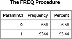
Figure 5.2 Percentage of Confidence Intervals That Contain the Parameter

For this simulation, 94.66% of the samples have a confidence interval that contains zero. For other values of the random seed, you might obtain 95.12% or 94.81%, but in general you should expect 95% of the confidence intervals to contain zero.
Exercise 5.1: Let P be the proportion of confidence intervals that contain zero. Rerun the program 10 times using 0 as the seed value, and record the range of values of P that you observe. Reduce the number of samples to 1,000 and run the new program 10 times. Compare the range of P values. Explain what you observe.
5.2.2 Coverage for Nonnormal Data
If the data are not normally distributed, then the interval ![]() contains the population mean with a probability that is different from 0.95. To demonstrate this, consider sampling from the standard exponential distribution, which has mean 1. In order to reuse the code from the previous section, subtract 1 from each observation in the sample so that the expected value of the population is zero, as shown here:
contains the population mean with a probability that is different from 0.95. To demonstrate this, consider sampling from the standard exponential distribution, which has mean 1. In order to reuse the code from the previous section, subtract 1 from each observation in the sample so that the expected value of the population is zero, as shown here:
data Exp;
   …
   x = rand(“Expo”) - 1;        /* x ~ Exp(1) - 1. Note E(X)=0 */
   …
run;
You can now use the Exp data set as the input for the MEANS procedure in the previous program. The percentage of confidence intervals that contain zero (the true mean) is no longer close to 95% (relative to the standard error) as shown in Figure 5.3.
Figure 5.3 Number of Intervals That Contain the True Mean for Exponential Data
For data drawn from the exponential data, the coverage probability is less than 95%. Simulation makes it easy to see that different data distributions affect the results of statistical methods.
Statisticians have developed exact confidence intervals for nonnormal distributions, including the exponential (Hahn and Meeker 1991).
Exercise 5.2: Produce Figure 5.3 by completing the details in this section.
Exercise 5.3: Use the BINOMIAL option on the TABLES statement to show that a 95% confidence interval about the estimate of 0.9344 does not include 0.95.
5.2.3 Computing Coverage in the SAS/IML Language
Section 5.2.1 uses simulation to estimate the coverage probability of the exact 95% confidence interval for normally distributed data. The following SAS/IML program repeats the analysis as a way of showing how to use the SAS/IML language for statistical simulation:
%let N = 50;                          /* size of each sample */
%let NumSamples = 10000;              /* number of samples   */
proc iml;
call randseed(321);
x = j(&N, &NumSamples);               /* each column is a sample    */
call randgen(x, “Normal”);            /* x ~ N(0,1)                 */

SampleMean = mean(x);                 /* mean of each column        */
s = std(x);                           /* std dev of each column     */
talpha = quantile(“t”, 0.975, &N-1);
Lower = SampleMean - talpha * s / sqrt(&N);
Upper = SampleMean + talpha * s / sqrt(&N);

ParamInCI = (Lower<0 & Upper>0);      /* indicator variable         */
PctInCI = ParamInCI[:];               /* pct that contain parameter */
print PctInCI;
Most statements are explained in the program comments. The RANDGEN routine generates a 50 × 10,000 matrix of standard normal variates. Each column is a sample. The MEAN and STD functions compute the mean and standard deviation, respectively, of each column. The QUANTILE function, which is described in Section 3.2, is used to compute the 1 − 0.05/2 quantile of the t distribution. Notice that SampleMean, s, Lower, and Upper are 1 × 10,000 row vectors. Consequently, ParamInCI is a 1 × 10,000 vector of zeros and ones. The colon operator (:) is used to compute the mean of the indicator variable, which is the proportion of ones. The results are displayed in Figure 5.4.
Figure 5.4 Proportion of Confidence Intervals That Contain the Parameter

Of the 10,000 samples of size 10, about 95% of them produce confidence intervals that contain zero.
Exercise 5.4: Repeat the SAS/IML analysis for exponentially distributed data.
5.3 Assessing the Two-Sample t Test for Equality of Means
A simple statistical test is the two-sample t test for the population means of two groups. There are several variations of the t test, but the pooled variance t test that is used in this section has three assumptions:
- The samples are drawn independently from their respective populations.
- The populations are normally distributed.
- The variances of the populations are equal.
In short, the t test assumes that samples are drawn independently from N(μ1, σ) and N(μ2, σ). The pooled variance t test enables you to use the sample data to test the null hypothesis that μ1 = μ2.
This section examines the robustness of the two-sample pooled-variance t test to the second and third assumptions. Similar analyses were conducted by Albert (2009, p. 12), Bailer (2010, p. 290), and Fan et al. (2002, p. 118).
5.3.1 Robustness of the t Test to Unequal Variances
This section uses simulation to study the sensitivity of the pooled-variance t test to the assumption of equal variances. The study consists of simulating data that satisfy the null hypothesis (μ1 = μ2) for the test. Consequently, it is a Type I error if the t test rejects the null hypothesis for these data. (Recall that a Type I error occurs when a null hypothesis is falsely rejected.)
For the remainder of this study, fix the significance level of the test at α = 0.05. Consider two scenarios. In the first scenario, the data are simulated from two N(0,1) populations. For these data, the populations have equal variances, and the probability of a Type I error is α. In the second scenario, one sample is drawn from an N(0,1) distribution whereas the other is drawn from N(0,10). Because the populations have different variances, the actual Type I error rate should be different from α.
The following DATA step generates 10,000 samples (each of size 10) from two populations. The classification variable, c, identifies the populations. The x1 variable contains the data for the first scenario; the x2 variable contains the data for the second scenario.
/* test sensitivity of t test to equal variances */
%let n1 = 10;
%let n2 = 10;
%let NumSamples = 10000;                /* number of samples       */

/* Scenario 1: (x1 | c=1) ~ N(0,1);  (x1 | c=2) ~ N(0,1);          */
/* Scenario 2: (x2 | c=1) ~ N(0,1);  (x2 | c=2) ~ N(0,10);         */
data EV(drop=i);
label x1 = “Normal data, same variance”
      x2 = “Normal data, different variance”;
call streaminit(321);
do SampleID = 1 to &NumSamples;
   c = 1;                               /* sample from first group */
   do i = 1 to &n1;
      x1 = rand(“Normal”);
      x2 = x1;
      output;
   end;
   c = 2;                               /* sample from second group */
   do i = 1 to &n2;
      x1 = rand(“Normal”);
      x2 = rand(“Normal”, 0, 10);
      output;
   end;
end;
run;
Notice the structure of the simulated data. The first 10 observations are for Group 1 (c = 1), the next 10 observations are for Group 2 (c = 2), and this pattern repeats as shown in Table 5.1. This structure is chosen because it also enables you to simulate data for which the number of observations in the two groups are not equal (see Exercise 5.7).
Table 5.1 Structure of the Simulated Data

In order to conduct the standard two-sample t test, you can call the TTEST procedure and use a BY statement to analyze each pair of samples. For each BY group, the TTEST procedure produces default output. However, to prevent thousands of pages of output, you should use ODS to suppress the output during the computation of the t statistics. In the following statements, the %ODSOFF macro is used to suppress output. The macro is described in Section 6.4.2. The ODS OUTPUT statement is used to write a data set that contains the p-value for each test.
/* 2. Compute statistics */
%ODSOff                        /* suppress output                 */
proc ttest data=EV;
   by SampleID;
   class c;                    /* compare c=1 to c=2              */
   var x1-x2;                  /* run t test on x1 and also on x2 */
   ods output ttests=TTests(where=(method=“Pooled”));
run;
%ODSOn                         /* enable output                   */
As shown in Section 5.2, you can use a DATA step to create a binary indicator variable that has the value 1 if the t test on the sample rejects the null hypothesis, and the value 0 if the t test does not reject the null hypothesis. You can use PROC FREQ to summarize the results, which are shown in Figure 5.5.
/* 3. Construct indicator var for tests that reject H0 at 0.05 significance */
data Results;
   set TTests;
   RejectH0 = (Probt <= 0.05);          /* H0: mu1 = mu2         */
run;

/* 3b. Compute proportion: (# that reject H0)/NumSamples */
proc sort data=Results;
   by Variable;
run;

proc freq data=Results;
   by Variable;
   tables RejectH0 / nocum;
run;
Figure 5.5 Summary of t Tests on 10,000 Samples, Normal Data
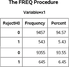
Figure 5.5 summarizes the results of the two scenarios. For the x1 variable (equal population variances), the t test rejects the null hypothesis for about 5% of the samples as predicted by theory. You can use the BINOMIAL option in the TABLES statement in PROC FREQ to assess the uncertainty in the simulation study. (See Exercise 5.5.)
For the x2 variable (unequal variances), 6.5% of the samples reject the null hypothesis. You should do additional simulation before you draw a conclusion, but this one simulation indicates that the t test rejects the null hypothesis more than 5% of the time when the population variances are not equal. Consequently, it is wise to use the Satterthwaite test rather than the pooled-variance test if you suspect unequal variances.
Exercise 5.5: Use the BINOMIAL option in the TABLES statement to compute a confidence interval for the proportion that the t test rejects the null hypothesis.
Exercise 5.6: The relative magnitudes of the population variances determine the proportion of samples in which the t test rejects the null hypothesis. Rerun the simulation when x2 (for c=2) is drawn from the N(0, 2), N(0, 5), and N(0,100) distributions. How sensitive is the pooled-variance t test to differences in the population variances?
Exercise 5.7: Rerun the simulation when the first sample (c=1) contains 20 observations and the second sample contains 10 observations. Compare the results with the results of a simulation in which both samples contain 15 observations. Which test has more power?
5.3.2 Robustness of the t Test to Nonnormal Populations
How sensitive is the two-sample pooled-variance t test to the assumption that both populations are normally distributed?
You can modify the program from Section 5.3.1 to sample from nonnormal distributions. For example, in one scenario you can draw samples from an exponential distribution for both the first group (c=1) and the second group (c=2). In another scenario, you can choose the first group from the normal distribution with unit standard deviation and the second group from an exponential distribution with a standard deviation 10 times as large. In each scenario, choose the population distributions so that the null hypothesis is true.
…
c = 1;
do i = 1 to &n1;
   x3 = rand(“Exponential”);               /* mean = StdDev = 1   */
   x4 = rand(“Normal”, 10);                /* mean=10; StdDev = 1 */
   output;
end;
c = 2;
do i = 1 to &n2;
   x3 = rand(“Exponential”);               /* mean = StdDev = 1   */
   x4 = 10 * rand(“Exponential”);          /* mean = StdDev = 10  */
   output;
end;
…
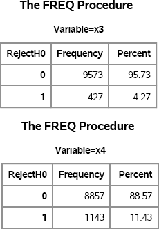
Figure 5.6 shows the results of t tests on the 10,000 samples. For the first scenario (both populations are Exp(1)), the test rejects the null hypothesis about 4.3% of the time. For the second scenario (one group is normal, the other is exponential, and the variances are unequal), the test rejects the null hypothesis about 11.4% of the time.
Figure 5.6 Summary of t Tests on 10,000 Samples, Nonnormal Data
One of the drawbacks of simulation is that it is difficult to generalize the results. Although it is clear that the t test rejects the null hypothesis for a large number of samples for the x4 variable, the simulation does not indicate why this is so. Is there something special about the exponential distribution, or would using a gamma or lognormal distribution give similar results? For the other tests, the distributions for each group are from the same family, but for x4 one sample is normally distributed whereas the other is exponentially distributed. Does that matter? Chapter 6, “Strategies for Efficient and Effective Simulation,” discusses these issues.
Exercise 5.8: Repeat the simulation for a new variable x5, which is drawn from a gamma(10) distribution when c = 1 and an exponential(10) distribution for c = 2. Both of these distributions have the same mean and variance, but both distributions are nonnormal. What percentage of the time does the t test reject the null hypothesis?
5.3.3 Assessing the t Test in SAS/IML Software
You can also investigate the robustness of the t test to its assumptions by using SAS/IML software. The formulas for the two-sample pooled variance t test are given in the documentation for the TTEST procedure in the SAS/STAT User's Guide. The following SAS/IML program reproduces the simulation of the x4 variable from Section 5.3.2 in which the first population is a normal distribution with unit standard deviation, and the second population is an exponential distribution with a standard deviation 10 times as large:
%let n1 = 10;
%let n2 = 10;
%let NumSamples = 1e4;              /* number of samples */

proc iml;
/* 1. Simulate the data by using RANDSEED and RANDGEN, */
call randseed(321);
x = j(&n1, &NumSamples);           /* allocate space for Group 1 */
y = j(&n2, &NumSamples);           /* allocate space for Group 2 */
call randgen(x, “Normal”, 10);     /* fill matrix from N(0,10)   */
call randgen(y, “Exponential”);    /* fill from Exp(1)           */
y = 10 * y;                        /* scale to Exp(10)           */

/* 2. Compute the t statistics; VAR operates on columns */
meanX = mean(x); varX = var(x);    /* mean & var of each sample  */
meanY = mean(y); varY = var(y);
/* compute pooled standard deviation from n1 and n2 */
poolStd = sqrt( ((&n1-1)*varX + (&n2-1)*varY)/(&n1+&n2-2) );

/* compute the t statistic */
t = (meanX - meanY) / (poolStd*sqrt(1/&n1 + 1/&n2));

/* 3. Construct indicator var for tests that reject H0 */
alpha = 0.05;
RejectH0 = (abs(t)>quantile(“t”, 1-alpha/2, &n1+&n2-2));   /* 0 or 1 */

/* 4. Compute proportion: (# that reject H0)/NumSamples */
Prob = RejectH0[:];
print Prob;
Figure 5.7 SAS/IML Summary of t Tests on 10,000 Samples, Nonnormal Data

In this program, the formula for the t test is explicitly used so that you can see how the SAS/IML language supports a natural syntax for implementing statistical methods. In the first part of the program, the RANDGEN subroutine generates all samples in a single call. Each column of the x matrix is a normal sample with 10 observations (rows). Similarly, each column of the y matrix is exponentially distributed. Notice that the SAS/IML approach does not use a classification variable, c. Instead, the observations with c=1 are stored in the matrix x, and the observations with c=2 are stored in the matrix y.
The second part of the program computes the sample statistics and stores them in the 1 × 10,000 vector t. All of the variables in this section are vectors. If you plan to use t tests often in PROC IML, then you can encapsulate these statements into a user-defined function.
The third part of the program compares the sample statistics with the (1 − α/2) quantile of the t distribution in order to generate an indicator variable, RejectH0. The colon subscript reduction operator (:) is used to find the mean of this vector, which is the proportion of elements that contains 1. This estimates the Type I error rate for the t test given the distribution of the populations. The error rate, which is displayed in Figure 5.7, is approximately 11%.
5.3.4 Summary of the t Test Simulations
The previous sections use simulation to examine the robustness of the two-sample pooled t test to normality and to equality of variances. The results indicate that the two-sample pooled t test is relatively robust to departures from normality but is sensitive to (large) unequal variances.
You can use the ideas in this chapter (and in the exercises) to build a large, systematic, simulation study that more carefully examines how the t test behaves when its assumptions are violated. Chapter 6 provides strategies for designing large simulation studies.
5.4 Evaluating the Power of the t Test
The simulations so far have explored how the two-sample t test performs when both samples are from populations with a common mean. That is, the simulations sample from populations that satisfy the null hypothesis of the test, which is μ1 = μ2, where μ1 and μ2 are the population means. A related question is, “How good is the t test at detecting differences in the population means?”
Suppose that μ2 = μ1 + δ, and, for simplicity, assume that the two populations are normally distributed with equal variance. When δ = 0, the population means are equal and the standard t test (with significance level α = 0.05) rejects the null hypothesis 5% of the time. If δ is larger than zero, then the t test should reject the null hypothesis more often. As δ gets quite large (relative to the standard deviation of the populations), the t test should reject the null hypothesis for almost every sample.
5.4.1 Exact Power Analysis
The power of the t test is the probability that the test will reject a null hypothesis that is, in fact, false. The power of the two-sample t test can be derived theoretically. In fact, the POWER procedure in SAS/STAT software can compute a “power curve” that shows how the power varies as a function of δ for normally distributed data:
proc power;
  twosamplemeans power = .        /* missing ==> “compute this” */
    meandiff= 0 to 2 by 0.1       /* delta =0, 0.1, …, 2        */
    stddev=1                      /* N(delta, 1)                */
    ntotal=20;                    /* 20 obs in the two samples  */
  plot x=effect markers=none;
  ods output Output=Power;        /* output results to data set */
run;
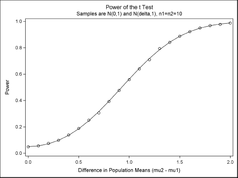
Figure 5.8 shows that when the means of the two groups of size 10 are two units apart (twice the standard deviation), the t test is almost certain to detect the difference in means. For means that are one unit apart (equal to the standard deviation), the chance of detecting the difference is about 56%. Of course, if the samples contain more than 10 observations, then the test can detect much smaller differences.
Figure 5.8 Power Curve for Two-Sample t Test, N1 = N2 = 10

5.4.2 A Simulated Power Analysis
Theoretical results for power computations are not always available. However, you can use simulation to approximate a power curve. This section uses simulation to estimate points along the power curve in Figure 5.8. To do this, use the techniques from Section 5.3 to sample from N(0,1) and N(δ,1) as δ varies from 0 to 2, and estimate the power for each value of δ. In particular, add a loop that iterates over the values of δ, as follows:
do Delta = 0 to 2 by 0.1;
   do SampleID = 1 to &NumSamples;
      …
      x1 = rand(“Normal”);            /* for c=1 */
      …
      x1 = rand(“Normal”, Delta, 1);  /* for c=2 */
      …
   end;
end;
Modify the call to PROC TTEST by adding the Delta variable to the list of BY variables:
by Delta SampleID;
You can then use PROC FREQ to estimate the power for each value of Delta. You can also combine these simulated estimates with the exact power values that are produced by PROC POWER in Section 5.4.1:
proc freq data=Results noprint;
   by Delta;
   tables RejectH0 / out=SimPower(where=(RejectH0=1));
run;

/* merge simulation estimates and values from PROC POWER */
data Combine;
   set SimPower Power;
   p = percent / 100;
   label p=“Power”;
run;

proc sgplot data=Combine noautolegend;
   title “Power of the t Test”;
   title2 “Samples are N(0, 1) and N(delta, 1), n1=n2=10”;
   series x=MeanDiff y=Power;
   scatter x=Delta y=p;
   xaxis label=“Difference in Population Means (mu2 - mu1)”;
run;
Figure 5.9 shows that the estimates obtained by the simulation with 10,000 samples are close to the exact values that are produced by PROC POWER. The simulation that creates Figure 5.9 is computationally intensive. It requires three nested loops in the DATA step and produces 21 × 10,000 × 20 = 4,200,000 observations and 210,000 t tests. Nevertheless, the entire simulation requires less than 30 seconds on a desktop PC that was manufactured in 2010.
Figure 5.9 Power Curve and Estimates from Simulation
Exercise 5.9: In Figure 5.9, each estimate is the proportion of times that a binary variable, RejectH0, equals 1. Use the BINOMIAL option in the TABLES statement in PROC FREQ to compute 95% confidence intervals for the proportion. Add these confidence intervals to Figure 5.9 by using the YERRORLOWER= option and YERRORUPPER= option in the SCATTER statement.
5.5 Effect of Sample Size on the Power of the t Test
The simulation in the previous section examines the power of the t test to reject the null hypothesis μ1 = μ2 for various magnitudes of the difference |μ1 − μ2|. Throughout the simulation, the sample sizes n1 and n2 are held constant. However, you can examine the power for various choices of the sample size for a constant magnitude of the difference between means, which is known as the effect size.
To be specific, suppose that the first group is a control group, whereas the second group is an experimental group. The researcher thinks that a treatment can increase the mean of the second group by 0.5. The researcher wants to investigate how large the sample size should be in order to have a power of 0.8. In other words, assuming that μ2 = μ1 + 0.5, what should the sample size be so that the null hypothesis is rejected (at the 5% significance level) 80% of the time?
This sort of simulation occurs often in clinical trials. Computationally, it is very similar to the previous power computation, and once again PROC POWER can provide a theoretical power curve. However, for many situations that are encountered in practice, theoretical results are not available and simulation provides a way to obtain the power curve as a function of the sample size.
For convenience, assume that both groups have the same sample size, n1 = n2 = N. The following simulation samples N observations from N(0, 1) and N(0.5, 1) populations for N = 40, 45,…, 100. For each value of the sample size, 1,000 samples are generated.
/* The null hypothesis for the t test is H0: mu1 = mu2.
   Assume that mu2 = mu1 + delta.
   Find sample size N that rejects H0 80% of the time.  */
%let NumSamples = 1000;            /* number of samples */

data PowerSizeSim(drop=i Delta);
call streaminit(321);
Delta =0.5;                        /* true difference between means */
do N = 40 to 100 by 5;             /* sample size                   */
   do SampleID = 1 to &NumSamples;
      do i = 1 to N;
         c = 1; x1 = rand(“Normal”);           output;
         c = 2; x1 = rand(“Normal”, Delta, 1); output;
      end;
   end;
end;
run;
This is a coarse grid of values for N. It is usually a good idea to do a small scale simulation on a coarse grid (and with a moderate number of samples) in order to narrow down the range of sample sizes. The remainder of the program is the same as in Section 5.4.2, except that you use the N variable in the BY statements instead of the Delta variable. The results are shown in Figure 5.10.
Figure 5.10 Power versus Sample Size
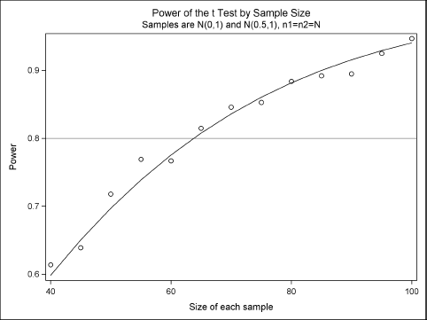
The markers in Figure 5.10 are the estimates of power obtained by the simulation. (You could also add binomial confidence intervals to the plot.) For this simple example, the exact results can be computed by using PROC POWER, so the exact power curve is overlaid on the estimates.
From an initial simulation on a coarse grid, about 65 subjects in each group are needed to obtain 80% power to detect a mean difference of 0.5. After you have narrowed down the possible range of sample sizes, you can decide whether you need to run a second, more accurate, simulation on a finer grid. For example, you might run a second simulation with N = 60, 61,…, 68 and with 10,000 samples for each value of N.
Exercise 5.10: Run a second simulation on a finer grid, using 10,000 samples for each value of N.
5.6 Using Simulation to Compute p-Values
An important use of simulations is the computation of p-values in hypothesis testing. To illustrate this technique, consider an experiment in which a six-sided die is tossed 36 times. The number of times that each face appeared is shown in Table 5.2:
Table 5.2 Frequency Count for Each Face of a Tossed Die

Suppose that you want to determine whether this die is fair based on these observed frequencies. The chi-square test is the usual way to test whether a set of observed frequencies are consistent with a specified theoretical distribution. For a given set of observed counts, Ni, the chi-square statistic is the quantity ![]() , where
, where ![]() .
.
To test whether the die is fair, the null hypothesis for the chi-square test is that the probability of each face appearing is 1/6. That is, P (X = i) = pi = 1/6 for i = 1,2,…, 6. Consequently, the observed value of the statistic for the data in Table 5.2 is q = 7.667.
The p-value is the probability under the null hypothesis that the random variable Q is greater than or equal to the observed value: PH0 (Q ≥ q). For large samples, the Q statistic has a χ2 distribution with k − 1 degrees of freedom, where k is the number of categories. (For a six-sided die, k = 6.) For small samples, you can use simulation to approximate the sampling distribution of Q under the null hypothesis. You can then estimate the p-value as the proportion of times that the test statistic, which is computed for simulated data, is greater than the observed value.
You can perform this computation using the SAS DATA step and the FREQ procedure, which performs chi-square tests. However, you can also perform the simulation by writing a SAS/IML program. The SAS/IML language supports the RANDMULTINOMIAL function, which generates random samples from a multinomial distribution (see Section 8.2). The counts for each face of a tossed die can be generated as a draw from the multinomial distribution: Each draw is a set of six integers, where the i th integer represents the number of times that the i th face appeared out of 36 tosses.
The SAS/IML implementation of the simulation is very compact:
proc iml;
Observed = {8 4 4 3 6 11};                     /* observed counts */
k = ncol(Observed);                            /*  6              */
N = sum(Observed);                             /* 36              */
p = j(1, k, 1/k);                              /* {1/6,…,1/6}     */
Expected = N*p; /* {6,6,…,6} */
qObs = sum( (Observed-Expected)##2/Expected ); /* q               */

/* simulate from null hypothesis */
NumSamples = 10000;
counts = RandMultinomial(NumSamples, N, p);    /* 10,000 samples */
Q = ((counts-Expected)##2/Expected )[ ,+];     /* sum each row   */
pval = sum(Q>=qObs) / NumSamples;              /* proportion > q */
print qObs pval;
Figure 5.11 Observed Value of χ2 Statistic and p-Value
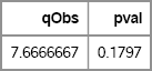
Figure 5.11 shows the observed value of the statistic and the proportion of simulated statistics (which were generated under the null hypothesis) that exceed the observed value. The simulation indicates that about 17% of the simulated samples result in a test statistic that exceeds the observed value. Consequently, the observed statistic is not highly unusual, and there is not sufficient evidence to reject the hypothesis of a fair die.
You can visualize the distribution of the test statistic and see where the observed statistic is located. The previous SAS/IML program did not end with a QUIT statement, so the following statements continue the program:
call symputx(“qObs”, qObs);                /* create macro variables */
call symputx(“pval”, pval);
create chi2 var {Q}; append; close chi2;
quit;
The statements use the SYMPUTX subroutine to create two macro variables that contain the value of qObs and pval, respectively. The simulated statistics are then written to a SAS data set. You can use the SGPLOT procedure to construct a histogram of the distribution, and you can use the REFLINE statement to indicate the location of the observed statistic. See Figure 5.12.
proc sgplot data=chi2;
   title “Distribution of Test Statistic under Null Hypothesis”;
   histogram Q / binstart=0 binwidth=1;
   refline &qObs / axis=x;
   inset “p-value = &pval”;
   xaxis label=“Test Statistic”;
run;
Figure 5.12 Approximate Sampling Distribution of the Test Statistic and Observed Value

If an observed statistic is in the extreme tail of the distribution, then the p-value is small. The INSET statement was used to include the value of the p-value in Figure 5.12.
Exercise 5.11: Construct a SAS data set with the data in Table 5.2 and run PROC FREQ. The CHISQ option in the TABLES statement conducts the usual chi-square test. Compare the p-value from the simulation to the p-value computed by PROC FREQ.
Exercise 5.12: Simulate 10,000 samples of 36 random values drawn uniformly from {1,2, 3, 4, 5, 6g. Use PROC FREQ with BY-group processing to compute the chi-square statistic for each sample. Output the OneWayChiSq table to a SAS data set. Construct a histogram of the chi-square statistics, which should look similar to Figure 5.12.
5.7 References
Albert, J. H. (2009), Bayesian Computation with R, 2nd Edition, New York: Springer-Verlag.
Bailer, J. (2010), Statistical Programming in SAS, Cary, NC: SAS Institute Inc.
Fan, X., Felsovályi, A., Sivo, S. A., and Keenan, S. C. (2002), SAS for Monte Carlo Studies: A Guide for Quantitative Researchers, Cary, NC: SAS Institute Inc.
Hahn, G. J. and Meeker, W. Q. (1991), Statistical Intervals: A Guide for Practitioners, New York: John Wiley & Sons.
Ross, S. M. (2006), Simulation, 4th Edition, Orlando, FL: Academic Press.