Chapter 13

Simulating Data from Time Series Models

Contents

13.1 Overview of Simulating Data from Time Series Models

Many processes can be modeled with time series. Applications of time series modeling include forecasting demand for retail goods, predicting seasonal fluctuations of airline passengers, and managing risk in financial portfolios. Simulation plays a big part in time series modeling. It is used to analyze the sensitivity of a model and to ask “What if” questions such as “What if there is a recession?” or “What if there is a stock market crash?”

A characteristic of time series is that the observations are correlated with each other. When you want to simulate univariate time series data, you need to modify the simulation techniques presented in Chapter 2, “Simulating Data from Common Univariate Distributions.” Whereas earlier chapters assumed that observation is drawn independently from a distribution, the techniques in this chapter simulate autocorrelated data. The autocorrelation of time series describes the correlation between values of the series at different time periods.

This chapter describes a few procedures and functions in SAS software that enable you to simulate data from time series. For univariate time series data, you can use either the DATA step or the ARMASIM function in SAS/IML software. To simulate multivariate time series data, use the SAS/IML VARMASIM function; it is unwieldy to use the DATA step for this purpose. Fan et al. (2002) present additional examples of simulating time series data with SAS software.

13.2 Simulating Data from Autoregressive and Moving Average (ARMA) Models

The regression models in Chapter 11, “Simulating Data for Basic Regression Models,” are useful when you want to examine the distribution of parameter estimates from SAS/STAT regression procedures such as PROC GLM and PROC MIXED. In a similar way, you can use simulated time series data to examine the sampling distributions of statistics that are produced by SAS/ETS procedures such as PROC ARIMA and PROC MODEL.

Two simple time series models are the autoregressive (AR) and the moving average (MA) models.

13.2.1 A Simple Autoregressive Model

In an AR model, the data are a series of observations where the value at time t is linearly related to the values at one or more previous times, plus a random error term. If ɸ₁, ɸ₂,…, are constants, then the AR model of order p (AR(p)) is as follows:

A particularly simple AR model assumes that the value at time t is related only to the value at the immediately preceding time. This is called an AR(1) model and has the form

y_t = ɸ₁y_t−1 + ∊_t

As is the case for linear regression, the error terms ∊_t are often chosen to be independent and to follow a normal distribution. The error terms are also called the innovations.

When simulating time series data, it suffices to simulate time series for which the series is expected to have zero mean and for which ∊_t ~ N(0,1). A simple linear transformation Z = σY + μ will transform the data to a series for which the expected mean is μ and for which ∊_t ~ N(0, σ).

13.2.2 Simulating AR(1) Data in the DATA Step

When simulating data from a stationary time series, a common technique is to generate a few values that are not recorded so that the initial value of the time series is not constant. This is shown in the following DATA step, which throws away 11 points before the simulated data are saved:

%let N = 100;
data AR1(keep=t y);
call streaminit(12345);
phi = 0.4; yLag = 0;
do t = -10 to &N;
   eps = rand(“Normal”);              /* variance of 1            */
   y = phi*yLag + eps;                /* expected value of Y is 0 */
   if t>0 then output;
   yLag = y;
end;
run;

You can visualize the time series and estimate the parameters by using the ARIMA procedure. The parameter estimates are shown in Figure 13.1.

ods graphics on;
proc arima data=AR1 plots(unpack only)=(series(corr));
   identify var=y nlag=1;                    /* estimate AR1 lag */
   estimate P=1;
   ods select SeriesPlot ParameterEstimates FitStatistics;
quit;

Figure 13.1 Parameter Estimates

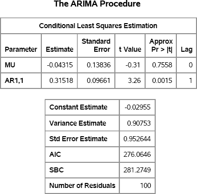
The series has three parameters. The expected value of the series is zero. The estimated value, MU, is shown in Figure 13.1. The estimate for MU is small and the corresponding p-value is large, which indicates that the data are consistent with the hypothesis that the parameter is zero.

The parameter estimate for ɸ is shown in the row with the AR1,1 heading. The parameter estimate is close to 0.4, which is the value assigned to the model.

The third parameter is the variance of the error term. The model uses a variance of 1, and the “Variance Estimate” row in Figure 13.1 shows that the estimated variance is close to its true value.

Figure 13.2 shows a plot of the time series. The plot indicates that the mean of the series is zero and that the standard deviation is approximately 1. Although is is difficult to estimate autocorrelation from this plot, you can see that an observation that is greater than zero (respectively, less than zero) tends to be followed by an observation that is also greater than zero (respectively, less than zero).

Exercise 13.1: In the DATA step, define Z = 3Y + 2. (Remember to add Z to the KEEP statement.) Run PROC ARIMA and specify VAR=Z in the IDENTIFY statement. How do the parameter estimates change?

Figure 13.2 Time Series for AR(1) Data

13.2.3 Approximating Sampling Distributions for the AR(1) Parameters

You can add a loop to the DATA step and use a BY statement in PROC ARIMA in order to approximate the sampling distributions of the statistics that are produced by PROC ARIMA. The PROC ARIMA statement does not support the NOPRINT option, but this option is supported in the IDENTIFY and ESTIMATE statements. The ESTIMATE statement also supports an OUTEST= option that creates an output data set. A WHERE clause is used to restrict the output to the three parameter estimates.

%let N = 100;
%let NumSamples = 1000;
/* simulate 1,000 time series from model */
data AR1Sim(keep=SampleID t y);
phi = 0.4;
call streaminit(12345);
do SampleID = 1 to &NumSamples;
   yLag = 0;
   do t = -10 to &N;
      y = phi*yLag + rand(“Normal”);
      if t>0 then output;
      yLag = y;
   end;
end;
run;

/* estimate AR(1) model for each simulated time series */
proc arima data=AR1Sim plots=none;
   by SampleID;
   identify var=y nlag=1 noprint;            /* estimate AR1 lag */
   estimate P=1 outest=AR1Est(where=(_TYPE_=“EST”)) noprint;
quit;

There are several ways to analyze the sampling distributions. The following statements use PROC UNIVARIATE to create a histogram (see Figure 13.3) of the approximate sampling distribution for the estimate of the ɸ parameter. The sampling distribution is asymptotically normal for large samples, so a normal curve is overlaid on the histogram. The MEANS procedure displays descriptive statistics, which are shown in Figure 13.4.

/* analyze sampling distribution */
ods graphics on;
proc univariate data=AR1Est;
   var AR1_1;
   histogram AR1_1 / normal;
   ods select histogram;
run;

proc means data=Ar1Est Mean Std P5 P95;
   var AR1_1;
run;

Figure 13.3 Approximate Sampling Distribution of AR(1) Parameter Estimate

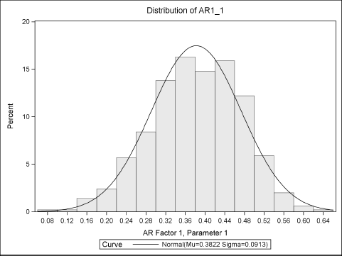
Figure 13.4 Descriptive Statistics of AR(1) Sampling Distribution

The standard deviation of the sampling distribution is the standard error of the parameter estimate. The Monte Carlo estimate in Figure 13.4 is similar to the estimate in Figure 13.1. However, the Monte Carlo standard error in Figure 13.4 is a better estimate than the point estimate in Figure 13.1, which was computed for a single time series with 100 observations.

Exercise 13.2: Visualize the sampling distribution of the variance of the error term and of the mean of the AR(1) process. Estimates for these quantities are in the ErrorVar and MU variables, respectively, in the AR1Est data set.

13.2.4 Simulating AR and MA Data in the DATA Step

In addition to the AR models, you can also simulate data from an MA model, or from a so-called ARMA model that combines the characteristics of the AR and MA models.

An MA model assumes that the error term at time t is linearly related to error terms at previous times. If θ₁, θ₂, …, θ_q are constants, then the MA model of order q (MA(q)) is as follows:

The SAS/ETS User's Guide cautions that “Moving-average errors can be difficult to estimate.” The documentation further notes that “A moving-average process can usually be well-approximated by an autoregressive process.”

The AR and MA models can be combined into a model that includes both kinds of terms. A general ARMA(p, q) model has the following form:

Again, the SAS/ETS User's Guide cautions that “ARMA models can be difficult to estimate,” and discusses issues that lead to “instability of the parameter estimates.”

Although checking the parameter estimates might be problematic, you can simulate data from an ARMA(p, q) model by using the DATA step. The following DATA step incorporates lagged effects by keeping previous values in an array. Although the program assumes that p > 0 and q > 0, you can easily modify the program to simulate, for example, data from a pure MA model. (Or simply set the AR coefficients to zero.)

/* simulate data from ARMA(p, q) model */
%let N = 5000;
%let p = 3;                                   /* order of AR terms */
%let q = 1;                                   /* order of MA terms */
data ARMASim(keep= t y);
call streaminit(12345);
array phi phi1 - phi&p (-0.6, 0, -0.3);       /* AR coefficients   */
array theta theta1 - theta&q ( 0.1);          /* MA coefficients   */
array yLag yLag1 - yLag&p;            /* save q lagged error terms */
array errLag errLag1 - errLag&q;      /* save p lagged values of y */

/* set initial values to zero */
do j = 1 to dim(yLag); yLag[j] = 0; end;
do j = 1 to dim(errLag); errLag[j] = 0; end;

/* “steady state” method: discard first 100 terms */
do t = -100 to &N;
   /* y_t is a function of values and errors at previous times      */
   e = rand(“Normal”);
   y = e;
   do j = 1 to dim(phi);                                  /* AR terms */
      y = y + phi[j] * yLag[j];
   end;
   do j = 1 to dim(theta);                               /* MA terms */
      y = y - theta[j] * errLag[j];
   end;
   if t > 0 then output;

   /* update arrays of lagged values */
   do j = dim(yLag) to 2 by -1; yLag[j] = yLag[j-1]; end;
   yLag[1] = y;
   do j = dim(errLag) to 2 by -1; errLag[j] = errLag[j-1]; end;
   errLag[1] = e;
end;
run;

The program is organized as follows:

1. The arrays phi and theta are used to hold the AR and MA coefficients, respectively.
2. The arrays yLag and errLag are used to hold the lagged values of the response and the error terms, respectively.
3. Zeros are assigned as initial values for all lagged terms. This is somewhat arbitrary, but it can be defended by noting that the series is assumed to have mean value 0 and the error terms also have mean value 0. Therefore, mean values are used in place of the unknown past values. However, notice that the p lagged values of Y do not have the correct autocovariance.
4. To make up for the fact that the initial values of Y do not have the correct autocovariance, the simulation discards the Y values for some initial period. In the program, “time” starts at t = −100, but data are not written to the data set until t > 0. By this time, the series should have settled into a steady state for which the response and error terms have the correct covariance.
5. The response at time t is computed according to the ARMA(p, q) model.
6. The arrays of lagged terms are updated.

You can use the SGPLOT procedure to visualize the stationary time series. The model depends on lags of order 1 and 3, so Figure 13.5 shows tick marks every 12 time periods.

proc sgplot data=ARMASim(obs=204);
   series x=t y=y;
   refline 0 / axis=y;
   xaxis values=(0 to 204 by 12);
run;

Figure 13.5 Simulated ARMA(3,1) Data

Exercise 13.3: Use PROC ARIMA analysis to estimate the AR and MA parameters. Because the series is so long (N = 5000), the parameter estimates are close to the model parameters. However, for short ARMA(p, q) time series this might not be the case.

Exercise 13.4: Rerun the simulation for N = 100, 500,1000, and 2000 and use PROC ARIMA to estimate the parameters, as was done in Section 13.2.3. Use PROC SGPLOT to plot the parameter estimates and standard errors as a function of the sample size.

13.2.5 Simulating AR(1) Data in SAS/IML Software

You can use the DATA step to simulate data from ARMA models, but it is much easier to use the ARMASIM function, which is part of SAS/IML software. The ARMASIM function simulates data from an AR, MA, or ARMA model.

The ARMASIM function uses a parameterization for the ARMA model in which the AR coefficients differ in sign from the formula in the previous section. The model used by the ARMASIM function has the following form:

where ɸ₀ = θ₀ = 1. There are other SAS/IML functions (such as ARMACOV and ARMALIK) that use the same parameterization.

An AR(1) time series with the same parameters as in Section 13.2.2 can be constructed as follows:

/* use the ARMASIM function to simulate a time series */
%let N = 100;
proc iml;
phi = {1 -0.4};    /* AR coefficients: Notice the negative sign!   */
theta = {1};       /* MA coefficients: Use {1, 0.1} to add MA term */
mu = 0;            /* mean of process                              */
sigma = 1;         /* std dev of process                           */
seed = -54321;     /* use negative seed if you call ARMASIM twice  */
yt = armasim(phi, theta, mu, sigma, &N, seed);

Notice that the second element in the phi vector has the opposite sign as the corresponding coefficient in the DATA step in Section 13.2.2. Also notice that the first elements in the phi and theta vectors are always 1 because they represent the coefficients of the y_t and ∊_t terms.

The ARMASIM function does not use the random number seed that is set by the RANDSEED subroutine (see Section 3.3). Instead, it maintains its own seed value. If you call ARMASIM twice with the same positive seed, then you will get exactly the same time series. In contrast, if you call ARMASIM twice with the same negative seed, then the second time series is different from the first, as shown by the following statements. The results are shown in Figure 13.6.

y1 = armasim(phi, theta, mu, sigma, 5,  12345)   /* 5 obs           */
y2 = armasim(phi, theta, mu, sigma, 5,  12345)   /* same 5 obs      */
y3 = armasim(phi, theta, mu, sigma, 5, -12345)   /* 5 obs           */
y4 = armasim(phi, theta, mu, sigma, 5, -12345)   /* different 5 obs */
print y1 y2 y3 y4;

Figure 13.6 Time Series with the Same Positive and Negative Seeds

In Figure 13.6, the vectors y1 and y2 have the exact same values, which is not usually very useful. However, the vectors y3 and y4, which use a negative seed value, have different values. Consequently, it is best to use a negative seed when you simulate an ARMA model.

You can use PROC IML to simulate multiple ARMA samples, as was done in Section 13.2.3. The following SAS/IML program generates the data and also creates a SampleID variable:

NumSamples = 1000;
Y = j(NumSamples, &N);
do i = 1 to NumSamples;
   z = armasim(phi, theta, mu, sigma, &N, -12345);   /* use seed < 0 */
   Y[i,] = z';                   /* put i_th time series in i_th row */
end;
SampleID = repeat(T(1:NumSamples),1,&N);
create AR1Sim var {SampleID Y}; append; close AR1Sim;
quit;

The program demonstrates a useful technique. Each simulated time series is stored in a row of the Y matrix. The SampleID matrix is a matrix of the same dimensions that has the value i for every element of the i th row. Recall that SAS/IML matrices are stored in row-major order. Therefore, when you use the CREATE statement and specify the SampleID and Y matrices, the elements of those matrices are written (in row-major order) to two long variables in the data set. There is no need to use the SHAPE function to create column vectors prior to writing the data.

Exercise 13.5: Create a SAS data set that contains the yt vector. Call PROC ARIMA and compare the parameter estimates to the estimates in Figure 13.1.

Exercise 13.6: Re-create Figure 13.3 and Figure 13.4 by using PROC ARIMA to analyze the Y variable in the AR1Sim data set. Mimic the PROC ARIMA code that is shown in Section 13.2.3.

13.3 Simulating Data from Multivariate ARMA Models

Fan et al. (2002) show examples of using the DATA step to simulate data from multivariate correlated time series where each component is simulated from an ARMA model. A multivariate time series of this type is known as a VARMA model.

The VARMA model includes matrices of parameters and vectors of response variables. Accordingly, simulating these data by using the DATA step requires writing out the matrix multiplication by hand. Fortunately, the SAS/IML language supports the VARMASIM subroutine, which has a syntax that is similar to the ARMASIM function.

For simplicity, consider a multivariate stationary VARMA(1,1) model with mean vector 0. If there are k components, then the VARMA(1,1) model is

y_t = Φy_t−1 + ∊_t − Θ∊_t−1

The k × k matrix Φ contains the AR coefficients. The (i, j)th element of Φ is the coefficient that shows how the i th component of y_t depends on the j th component of y_t−1. The vector ∊_t (the vector of innovations) is assumed to be multivariate normal with mean vector 0 and k × k covariance matrix Σ. The k × k matrix Θ contains the MA coefficients.

The following SAS/IML program simulates a trivariate (k = 3) stationary time series that has no MA coefficients (Θ = 0). The errors have covariance given by the matrix Σ, and the AR coefficients are given by the Phi matrix.

proc iml;
Phi = {0.70 0.00 0.00,               /* AR coefficients      */
       0.30 0.60 0.00,
       0.10 0.20 0.50};
Theta = j(3,3,0);                    /* MA coefficients = 0  */
mu = {0,0,0};                        /* mean = 0             */
sigma = {1.0 0.4 0.16,               /* covariance of errors */
         0.4 1.0 0.4,
         0.16 0.4 1.0};
call varmasim(y, Phi, Theta, mu, sigma, &N) seed=54321;

create MVAR1 from y[colname={“y1” “y2” “y3”}];
append from y;
close MVAR1;
quit;

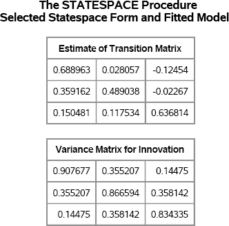
To verify that the simulated data are from the specified model, you can use the STATESPACE procedure to estimate the parameters and covariances. Figure 13.7 shows the parameter estimates for the AR coefficients and the covariance of the error terms (innovations) based on 100 simulated observations. The estimates of the AR coefficients are contained in the “Estimates of Transition Matrix” table. The estimates are somewhat close to the model parameters, except for the Φ₁₃ parameter. The covariance estimates are also reasonably close but, as you might guess, the standard errors for these statistics are large when the time series contains only 100 observations.

proc statespace data=MVAR1 interval=day armax=1 lagmax=1;
   var y1−y3;
   ods select FittedModel.TransitionMatrix FittedModel.VarInnov;
run;

Figure 13.7 Multivariate AR(1) Time Series with Correlated Innovations

Exercise 13.7: Simulate 1,000 data samples from the VARMA model. Analyze the results with PROC STATESPACE and compute estimates for the standard errors of the AR coefficients and the elements of the innovation covariance.

13.4 References

Fan, X., Felsovályi, A., Sivo, S. A., and Keenan, S. C. (2002), SAS for Monte Carlo Studies: A Guide for Quantitative Researchers, Cary, NC: SAS Institute Inc.