Chapter 16

Moment Matching and the Moment-Ratio Diagram

Contents

16.1 Overview of Simulating Data with Given Moments

Given data, how can you simulate additional samples that have the same distributional properties? There are several techniques:

• You can sample from the empirical distribution of the data, which is precisely the basic bootstrap algorithm, as discussed in Chapter 15, “Resampling and Bootstrap Methods.”
• You can use a well-known “named” parametric distribution to model the data. You can then simulate the data by drawing random samples from the fitted distribution.
• You can model the data as a finite mixture of distributions. The FMM procedure in SAS/STAT software can fit a wide range of mixture models to data. After you have fit a model, you can use the ideas in Section 7.5 to simulate data from the model.
• For univariate data, you can choose a flexible system of distributions such as the Pearson system (Ord 2005), the Burr system (Burr 1942; Rodriguez 2005), or the Johnson system (Johnson 1949; Bowman and Shenton 1983; Slifker and Shapiro 1980).
• You can use Fleishman's method (Fleishman 1978) and its multivariate generalization (Vale and Maurelli 1983) to construct a distribution whose population mean, variance, skewness, and kurtosis match the corresponding sample statistics for the data.

These approaches are summarized in Figure 16.1. This chapter describes how to use the Johnson system and the Fleishman transformation; the other methods have been discussed previously. Tadikamalla (1980) gives a concise summary of the advantages and disadvantages of the Johnson system and the Fleishman transformation.

Figure 16.1 Some Methods to Simulate from Observed Data

The idea of simulating data from a parametric distribution whose mean, variance, skewness, and kurtosis match the corresponding sample statistics for the data is called moment matching. This chapter describes how to use moment matching to simulate data from a distribution with a specified mean, variance, skewness, and kurtosis.

This chapter also describes a useful graphical tool, called the moment-ratio diagram. This diagram can help you to select candidate distributions to model the data and to compare simulations from different distributions. Traditionally the moment-ratio diagram is a theoretical tool for understanding the relationships of families and systems of distributions. This chapter shows how to use the moment-ratio diagram as a tool to organize simulation studies.

16.2 Moments and Moment Ratios

The moments of a distribution measure aspects of the distribution's location, scale, and shape. For a random variable X, let μ be the mean, which is the first (raw) moment. The central moment of order r is μ_r = E((X – μ)^r), where E denotes the expected value operator. For example, the second central moment is the variance of the distribution, μ₂ = σ².

The skewness and kurtosis are the third and fourth standardized central moments, respectively. The word “standardized” indicates that the deviation about the mean is divided by the standard deviation. The skewness is defined as

and the kurtosis is defined as

Because the skewness and kurtosis are ratios of centralized moments, they are referred to as moment ratios. The kurtosis of the normal distribution is 3, so many researchers use the quantity k – 3, which is known as the excess kurtosis or the coefficient of excess. In fact, many references drop the “excess” modifier altogether. For example, the statistic labeled “kurtosis” in the output of SAS procedures is actually an estimate of the excess kurtosis. When there is no chance for confusion, this book uses “kurtosis” to mean excess kurtosis. When clarity is needed, the modifiers “full” or “excess” are used.

In this chapter, the adjectives “central” and “standardized” are usually dropped and the phrase “the first four moments” is sometimes used to refer to the mean, variance, skewness, and kurtosis of a distribution.

Of course, there are sample statistics that estimate these quantities. The formulas that SAS uses are the same as in Kendall and Stuart (1977) and are given in the appendix “SAS Elementary Statistics Procedures” in the Base SAS Procedures Guide. A SAS/IML program that computes estimates is included in this book in Appendix A, “A SAS/IML Primer.”

16.3 The Moment-Ratio Diagram

The moment-ratio diagram (Johnson, Kotz, and Balakrishnan 1994) shows the relationship between the skewness and the kurtosis for any univariate family of distributions for which the first four moments exist.

Many families include parameters (called shape parameters) that change the skewness (γ) and full kurtosis (k) of the distribution. By plotting the locus of (γ, k) values as the shape parameters vary over their possible values, you can visualize the relationship between the skewness and kurtosis for each distribution. (In some references, the locus of (γ², k) values is plotted instead.)

By convention, the moment-ratio diagram is shown “upside down,” with the kurtosis axis pointing down. Also by convention, the full kurtosis, k, is shown rather than the excess kurtosis, k – 3. For convenience, the diagrams in this book include axes for both the full kurtosis and the excess kurtosis.

The theoretical skewness and kurtosis of a distribution cannot take on arbitrary values. The kurtosis and skewness must obey the relationship k ≥ 1 + γ². This defines the feasible region.

Table 16.1 shows the skewness and excess kurtosis for a small set of continuous distribution. The moment-ratios for these distributions are shown in Figure 16.2.

Table 16.1 Skewness and Excess Kurtosis for Some Continuous Distributions

Figure 16.2 Moment-Ratio Diagram for Some Continuous Distributions

Figure 16.2 graphically demonstrates the following facts about the distributions in Table 16.1:

• The normal, Gumbel, and exponential distributions have no shape parameters. They are represented in the moment-ratio diagram as points labeled N, G, and E, respectively.
• The t distribution has a discrete shape parameter: the degrees of freedom. The t family is represented as a sequence of points that converges to the normal distribution. Like all symmetric distributions, these points lie along the γ = 0 axis.
• The lognormal and gamma distributions have one shape parameter and are represented as curves. For example, the locus of points for the gamma distribution (the upper curve at the edge of the beta region) is the parametric curve (2/ 6/α) for α > 0.
• The beta distribution has two shape parameters. It is represented by a region in the moment-ratio diagram.

The moment-ratio diagram is drawn by using the annotation facility of the SGPLOT procedure, which was introduced in SAS 9.3. You can use the annotation facility to draw arbitrary curves, regions, and text on a graph that is created by PROC SGPLOT. This book's Web site contains SAS programs that display the moment-ratio diagram for continuous distributions.

Figure 16.2 contains two vertical axes. The axis on the left indicates the excess kurtosis, whereas the axis on the right indicates the full kurtosis, k. By convention, the axes point down.

Notice that the moment-ratio diagram does not fully describe a distribution because only the skewness and kurtosis are represented. For example, the fact that the Gumbel distribution lies on the lognormal curve does not imply that the Gumbel distribution is a member of the lognormal family, only that the distributions have the same skewness and kurtosis for some lognormal parameter value.

Figure 16.2 is a simple moment-ratio diagram. Vargo, Pasupathy, and Leemis (2010) present a more comprehensive moment-ratio diagram that includes 37 different distributions. The applications in this chapter do not require this complexity, but the diagram is reproduced in Figure 16.3 so that you can appreciate its beauty. The figure is reprinted with permission from the Journal of Quality Technology©2010 American Society for Quality. No further distribution allowed without permission.

Exercise 16.1: Show that the Bernoulli distribution with parameter p exactly satisfies the equation k = 1 + γ². In this sense, the Bernoulli distribution has the property that its kurtosis is as small as possible given its skewness.

Exercise 16.2: The moment ratios for the Gamma(4) distribution are close to those of the Gumbel family. Plot the density of the Gamma(4) distribution and compare its shape to that of several Gumbel densities. The PDF of the Gumbel(μ, σ) distribution is f(x) = exp(–z – exp(–z))/σ, where z = (x – μ)/σ.

Figure 16.3 Comprehensive Moment-Ratio Diagram

16.4 Moment Matching As a Modeling Tool

The problem of finding a flexible family (or system) of distributions that can fit a wide variety of distributional shapes is as old as the study of statistics. Between 1895 and 1916, Karl Pearson constructed a system of seven families of distributions that model data. Given a valid combination of the first four sample moments, the Pearson system provides a family that matches these four moments. Although the Pearson system is valuable for theory, practitioners prefer systems with fewer families such as the Johnson system.

A drawback of these systems is that they cannot be used to fit all distributions. They are primarily useful for fitting unimodal distributions, although the Johnson system and other parametric models can also be used to fit some bimodal distributions.

Although some modelers now favor nonparametric techniques, parametric families of distributions offer certain advantages such as the ability to fit a distributional form that involves a small number of parameters, some of which might have a practical interpretation. Consequently, the practice of fitting parametric distributions to data is still popular.

Moment matching is an attempt to match the shape of data by using four parameters that are easy to compute and relatively easy to interpret. The mean and variance estimate the expected value and the spread of the data, respectively. The skewness describes the asymmetry of the data. Positive skewness indicates that data are more prevalent in the right tail than in the left tail. The kurtosis is less intuitive, but for unimodal distributions it is generally interpreted as describing whether the distribution has a sharp peak and long tails (high kurtosis) or a low wide peak and short tails (low kurtosis).

Because the first two moments do not affect the shape of the data, the rest of this chapter is primarily concerned with finding distributions with a given skewness and kurtosis. If you use moment matching for small samples, keep in mind that “the estimates of these moments are highly biased for small samples” (Slifker and Shapiro 1980), and that they are very sensitive to outliers.

16.5 Plotting Variation of Skewness and Kurtosis on a Moment-Ratio Diagram

Now that the moment-ratio diagram has been explained, how can you apply it to the problem of simulating data? One application is to use the diagram to “identify likely candidate distributions” for data (Vargo, Pasupathy, and Leemis 2010, p. 6).

The simplest way to use the moment-ratio diagram is to locate the sample skewness and kurtosis of observed data on the diagram, and then look for “nearby” theoretical distributions. However, it is often not clear which distributions are “nearby” and which distributions are “far away.” Nearness depends on the standard errors of the sample skewness and kurtosis. You can use bootstrap techniques to estimate the standard errors as shown in Section 15.3.

16.5.1 Example Data

The following DATA step creates 200 positive “observed” values that are used in this and subsequent sections. (Full disclosure: These data are fake.) Figure 16.4 shows summary statistics and Figure 16.5 shows a histogram and kernel density estimate of the data.

data MRData;
input x @@;
datalines;
  4.54 4.57 7.18 5.03 3.70  4.11 2.79 2.30 1.75 2.08 1.70 4.83 4.57 11.51
  2.36 6.47 3.86 7.14 6.96  3.59 5.81 5.66 7.07 2.29 4.42 1.01 6.49  2.59
  5.36 3.90 6.50 4.97 5.29  4.83 4.62 3.04 3.67 3.68 4.09 4.95 1.66  4.07
  4.31 2.20 2.29 6.38 3.58  4.11 2.50 2.94 1.47 6.77 9.54 2.14 2.84  3.25
  2.65 5.62 4.41 1.18 3.76  0.95 4.67 5.17 1.08 4.09 2.84 1.96 6.23  3.48
  5.41 6.17 7.71 2.84 2.32  4.40 3.21 2.22 0.56 3.53 3.03 1.35 1.97  1.61
  3.02 2.49 4.06 2.82 6.22 13.18 4.04 3.56 3.65 2.48 3.90 3.44 5.11  3.93
  1.69 6.12 2.75 4.60 5.97  1.75 2.01 4.02 2.34 7.20 0.69 3.10 3.92 11.71
  1.56 3.03 4.01 2.61 2.88  5.97 6.24 7.89 5.11 3.36 1.56 7.50 2.16  1.33
  1.42 2.76 2.17 3.41 3.47  3.15 4.08 2.29 3.95 5.42 1.77 2.80 9.69  3.95
  9.04 1.38 2.61 1.14 5.24  1.42 2.06 5.46 3.72 9.80 2.77 1.71 7.25  2.86
  5.15 2.94 3.00 1.90 4.61  3.64 7.54 1.85 2.50 0.95 1.14 1.85 3.97  6.06
  4.47 6.69 2.02 6.04 5.63  5.17 2.12 3.70 1.72 3.50 3.73 8.03 6.87  5.01
  1.07 5.17 4.97 2.99 2.45  5.82 5.50 5.34 4.65 4.73 2.91 4.75 1.45  4.27
  3.71 3.16 5.82 6.24
;

proc means data=MRData N min max mean std skew kurt maxdec=3;
run;

proc univariate data=MRData;
   histogram x / midpoints=(0 to 13);
   ods select Histogram;
run;

Figure 16.4 Summary Statistics

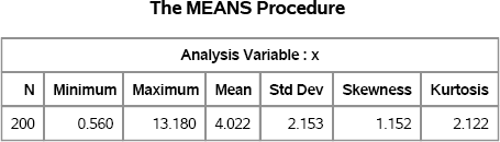
Figure 16.5 Histogram of Sample

As shown in Figure 16.1, there are various ways to produce simulated samples that match the characteristics of the observed data. For each technique, you can plot the skewness and kurtosis of the simulated samples on the moment-ratio diagram. This enables you to visually assess the sampling variability of these statistics.

16.5.2 Plotting Bootstrap Estimates of Standard Errors

The following statements use the basic bootstrap technique to generate 100 samples (technically resamples) of the MRData data set. The estimates of skewness and kurtosis for each bootstrap sample are plotted on the moment-ratio diagram in Figure 16.6. Reference lines are added to show the skewness and kurtosis values of the observed data. The macro that creates the moment-ratio diagram is available from this book's Web site.

/* use SURVEYSELECT to generate bootstrap resamples */
proc surveyselect data=MRData out=BootSamp noprint
     seed=12345 method=urs rep=100 rate=1;
run;

proc means data=BootSamp noprint;
   by Replicate;
   freq NumberHits;
   var x;
   output out=MomentsBoot skew=Skew kurt=Kurt;
run;

title “Moment-Ratio Diagram”;
title2 “100 Bootstrap Resamples, N=200”;
%PlotMRDiagramRef(MomentsBoot, anno, Transparency=0.4);

Figure 16.6 Skewness and Kurtosis of Bootstrap Resamples

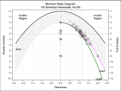
Vargo, Pasupathy, and Leemis (2010) suggest using the spread of the moment-ratio “cloud” to guide the selection of a model. A candidate distribution is one that is close to the center of the cloud. (You can also fit a bivariate normal predicton ellipse to the points of the cloud; see Vargo, Pasupathy, and Leemis (2010) for an example.)

For the current example, plausible candidates include the gamma distribution, the Gumbel distribution, and the lognormal families. The next section explores simulating the data with a fitted gamma distribution.

Exercise 16.3: Use the HISTOGRAM statement in PROC UNIVARIATE to estimate parameters for the candidate distributions and overlay the density distributions. Read the next section if you need help fitting distributions to the data.

16.6 Fitting a Gamma Distribution to Data

Suppose that you decide to use a gamma family to fit to the MRData data. This decision might be motivated by some domain-specific knowledge about the data, or it might be made by noticing that the sample moment-ratios in Figure 16.6 lie along the curve for the gamma family.

You can use the UNIVARIATE procedure to fit a gamma distribution to the data. The UNIVARIATE procedure uses a generalization of the gamma distribution that includes a threshold and scale parameter. The following statements set the threshold parameter to zero and fit the scale and shape parameters. The parameter estimates are shown in Figure 16.7. The INSET statement is used to display the skewness and kurtosis values on the histogram, which is shown in Figure 16.8.

proc univariate data=MRData;
   var x;
   histogram x / gamma(theta=0);
   inset skewness kurtosis / format=5.3;
   ods select Histogram ParameterEstimates;
run;

Figure 16.7 Parameter Estimates for a Gamma Distribution

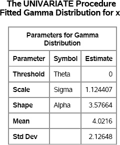
Figure 16.7 shows the parameter estimates for the scale and shape parameters, which are computed by using maximum likelihood (ML) estimation. The mean and standard deviation of the fitted distribution are also displayed. Goodness-of-fit statistics are not shown but indicate that the fit is good. As shown in Table 16.1, the skewness of a gamma distribution with shape parameter α = 3.58 is 2/ = 1.06, and the excess kurtosis is 6/3.58 = 1.68. Notice that these ML estimates do not match the sample skewness and kurtosis, which is to be expected. (An alternative approach would be to find the value of α such that (2/ 6/α) is closest to the sample skewness and kurtosis.)

Figure 16.8 Distribution of Data with Fitted Gamma Density

The model fitting is complete. You can now simulate from the fitted model.

An interesting application of the moment-ratio diagram is to assess the variability of the skewness and kurtosis of the simulated samples. Figure 16.6 shows the variability in those statistics for the original data as estimated by the bootstrap method. Does simulating from the fitted gamma distribution lead to a similar picture?

The following DATA step simulates the data from the fitted gamma model and computes the skewness and kurtosis for each sample. These values are overlaid on the moment-ratio diagram in Figure 16.9.

%let N = 200;                               /* match the sample size */
%let NumSamples = 100;
data Gamma(keep=x SampleID);
call streaminit(12345);
do SampleID = 1 to &NumSamples;
   do i = 1 to &N;
      x = 1.12 * rand(“Gamma”, 3.58);
      output;
   end;
end;
run;

proc means data=Gamma noprint;
   by SampleID;
   var x;
   output out=MomentsGamma mean=Mean var=Var skew=Skew kurt=Kurt;
run;

title “Moment-Ratio Diagram”;
title2 “&NumSamples Samples from Fitted Gamma, N=&N”;
%PlotMRDiagramRef(MomentsGamma, anno, Transparency=0.4);

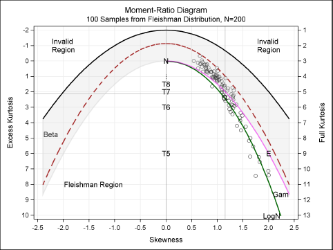
Figure 16.9 Skewness and Kurtosis of Simulated Samples: Gamma Model

Figure 16.9 shows the skewness-kurtosis values for each sample of size 200. Again, reference lines show the skewness and kurtosis values of the observed data. Figure 16.9 looks similar to Figure 16.6, although the dispersion of the cloud for the gamma model appears to be greater than for the bootstrap cloud. The sample skewness ranges from 0.4 to 1.9, and the excess kurtosis ranges from –0.6 to 6.8.

Exercise 16.4: An advantage of a parametric model is that you can simulate different sample sizes. Rerun the simulation with N = 10,000 observations in each sample. Create a scatter plot of the sample skewness and kurtosis for each simulation. (You do not need to overlay the moment-ratio diagram.) What do you observe about the size of the cloud?

Exercise 16.5: Use PROC UNIVARIATE to fit a Gumbel distribution to the data. Simulate 100 random samples from the fitted Gumbel distribution, each containing 200 observations. (See Section 7.3 for how to simulate Gumbel data.) Create a scatter plot of the sample skewness and kurtosis for the simulated data and compare it to Figure 16.9.

16.7 The Johnson System

The previous section assumes that the gamma distribution is an appropriate model for the data. However, sometimes you simply do not know whether any “named” family is appropriate for a given set of data. In that case, you might turn to a flexible system of distributions that can be used to fit a wider variety of distributional shapes.

Johnson's system (Johnson 1949) consists of three families of distributions that are defined by normalizing transformations: the S_B distributions, the S_L distributions (which are the lognormal distributions), and the S_U distributions. Section 7.3.7 and Section 7.3.8 discuss the distributions and provide DATA steps that simulate data from them.

Together, these distributions (and the normal distribution) cover the range of valid moment ratios as described in Section 16.3. Figure 16.10 shows that the lognormal distribution (and its reflection) separates the moment-ratio diagram into two regions. Distributions in the upper region have relatively low kurtosis. Each (γ, k) value in the upper region is achieved by one S_B distribution. The lower region corresponds to high kurtosis values. Each (γ, k) value in the lower region is achieved by one S_U distribution.

Figure 16.10 Moment Ratios for the Johnson System of Distributions

The sample moment ratios for the MRData data are in the S_B region. The UNIVARIATE procedure can use the first four sample moments to fit a family in the Johnson system. Be aware, however, that the variances of the estimates of the third and fourth moments are quite high, that the estimates are biased for small samples, and that the estimates are not robust to outliers (Slifker and Shapiro 1980). The following statements use the method of moments to fit the S_B family to the MRData data. Figure 16.11 shows the parameter estimates and the associated moments for the S_B distribution. The UNIVARIATE procedure does not provide goodness-of-fit statistics for the S_B family, but Figure 16.12 indicates that the model appears to fit the data well.

proc univariate data=MRData;
   var x;
   histogram x / sb(fitmethod=Moments theta=est sigma=est);
   ods output ParameterEstimates=PE;
   ods select Histogram ParameterEstimates;
run;

Figure 16.11 Parameter Estimates for a S_B Distribution

Figure 16.12 Distribution of Data with Fitted S_B Density

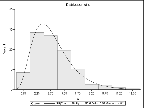
The model fitting is complete. You can now simulate from the fitted model as described in Section 7.3.7. You can use the moment-ratio diagram to assess the variability of the skewness and kurtosis of the simulated samples. Figure 16.13 displays the cloud of the sample skewness and kurtosis values. The cloud is similar to Figure 16.9 and includes reference lines that show the skewness and kurtosis of the observed data.

Figure 16.13 Skewness and Kurtosis of Simulated Samples: Johnson S_B Distribution

16.8 Fleishman's Method

Fleishman (1978) uses a cubic transformation of a standard normal variable to construct a distribution with given moments. The transformation starts with a standard normal random variable, Z, and generates a new random variable defined by the polynomial

Y = c₀ + c₁Z + c₂Z² + c₃Z³

Given specific values of skewness and kurtosis, you can often (but not always) find coefficients so that Y has the given skewness and kurtosis. Fleishman (1978) tabulated coefficient values (always setting c₀ = –c₂) for selected values of skewness and kurtosis. Alternatively, many researchers (for example, Fan et al. (2002)) use root-finding techniques to solve numerically for the coefficients that give specified values of skewness and kurtosis.

For years there were two main objections to using Fleishman's method (Tadikamalla 1980):

• For a given value of skewness, γ, there are distributions with (full) kurtosis k for all k ≥ 1 + γ². However, the distributions that are generated by using Fleishman's transformation cannot achieve certain low values of kurtosis. In particular, Fleishman distributions are bounded by the equation k ≥ 1.8683 + 1.58837γ².
• The distribution of Y was not known in terms of an analytic expression. Although it was possible to generate random samples from Y, quantiles, modes, and other important features were not available.

Figure 16.14 shows the region k ≥ 1.8683 + 1.58837γ² that can be achieved by cubic transformations of a standard normal variate. Any (γ, k) value below the dashed curve can be generated by Fleishman's transformation.

Figure 16.14 Moment-Ratio Diagram with Fleishman Region

Today, however, these objections are less troublesome thanks to recent research that was primarily performed by Todd Headricks and his colleagues.

• Fleishman's cubic transformation method has been extended to higher-order polynomials (Headrick 2002, 2010) and is now the simplest example of the general “power transformation” method of generating nonnormal distributions. Using higher-order polynomials decreases (but does not eliminate) the region of unobtainable (γ, k) values at the cost of solving more complicated equations.
• Headrick and Kowalchuk (2007) published a description of the PDF and CDF for the power transformation method.

Fleishman's method is often used in practice because it is fast, relatively easy, and it extends to multivariate correlated data (Vale and Maurelli 1983). Headrick (2010) is the authoritative reference on the properties of Fleishman's transformation.

This book's Web site contains a series of SAS/IML functions that you can use to find the coefficients of Fleishman's cubic transformation for any obtainable skewness and kurtosis values. You can download and store the functions in a SAS/IML library, and use the LOAD statement to read the modules into the active PROC IML session.

There are three important SAS/IML functions for using the Fleishman method:

• The MOMENTS module, which computes the sample mean, variance, skewness, and kurtosis for each column of an N × p matrix.
• The FITFLEISHMAN module, which returns a vector of coefficients {c₀, c₁, c₂, c₃} that transforms the standard normal distribution into a distribution (the Fleishman distribution) that has the same moment ratios as the data.
• The RANDFLEISHMAN module, which generates an N × p matrix of random variates from the Fleishman distribution, given the coefficients {c₀, c₁, c₂, c₃}.

The following SAS/IML program reads the MRData data and finds the cubic coefficients for the Fleishman transformation. As in previous sections, you can simulate 100 samples from the Fleishman distribution that has the same skewness and kurtosis as the data and plot the moment-ratios, as shown in Figure 16.15.

/* Define and store the Fleishman modules */
%include “C:<path>RandFleishman.sas”;

/* Use Fleishman's cubic transformation to model data */
proc iml;
load module=_all_;                         /* load Fleishman modules */
use MRData;  read all var {x};  close MRData;

c = FitFleishman(x);       /* fit model to data; obtain coefficients */

/* Simulate 100 samples, each with nrow(x) observations */
call randseed(12345);
Y = RandFleishman(nrow(x), 100, c);
Y = mean(x) + std(x) * Y;                   /* translate and scale Y */

varNames = {“Mean” “Var” “Skew” “Kurt”};
m = T( Moments(Y) );
create MomentsF from m[c=varNames];  append from m;  close MomentsF;
quit;

title “Moment-Ratio Diagram”;
title2 “&NumSamples Samples from Fleishman Distribution, N=&N”;
%PlotMRDiagramRef(MomentsF, Fanno, Transparency=0.4);

Figure 16.15 shows the sample skewness and kurtosis of 100 samples that are generated by using a cubic transformation of normal variates. Reference lines show the skewness and kurtosis values of the observed data. Notice that all moment ratios are inside the Fleishman region, which is indicated by the dashed parabola. The variability of the moment-ratios appears to be similar to that shown in Figure 16.13 for the Johnson family.

When matching moments to data, there are an infinite number of distributions that give the same set of moments. The Johnson family and the Fleishman transformation are two useful techniques to simulate data when the first four moments are specified. Because four moments do not completely characterize a distribution, you should always plot a histogram of a simulated sample as a check that the model is appropriate for the data.

Figure 16.15 Skewness and Kurtosis of Simulated Samples: Fleishman Distribution

16.9 Comparing Simulations and Choosing Models

As shown in the previous sections, the moment-ratio diagram enables you to compare simulations from different models. When you present the results of a simulation study, be sure to explain the details of the study so that others can reproduce, extend, or critique the methods used.

Section 16.6 fits a model from the gamma distribution and simulates data from the fitted model. This is the usual approach: You choose a parametric family and use the data to estimate the parameters. As shown in Section 16.5, you can use the moment-ratio diagram to help choose candidates for modeling.

Section 16.7 and Section 16.8 uses a moment-matching approach to fit the data. The Johnson system and the Fleishman transformation are flexible tools that can fit a wide range of distribution shapes.

The Johnson system can be used to fit any feasible pair of skewness and kurtosis values. However, it is not always easy to fit a Johnson distribution to data. The Fleishman transformation is not quite as flexible, but has the advantage of being a single method rather than a system of three separate distributions. You can use the programs from this book's Web site to generate samples from distributions that have specified moments.

No matter what method you use to simulate data, you can use the moment-ratio diagram to assess the variability of the sample skewness and kurtosis.

16.10  The Moment-Ratio Diagram As a Tool for Designing Simulation Studies

In addition to its usefulness as a modeling tool, moment matching is a valuable technique that you can use to systematically simulate data from a wide range of distributional shapes.

Imagine that you want to use simulation to explore how a statistic or statistical technique behaves for nonnormal data. A well-designed simulation study should choose distributions that are representative of the variety of nonnormal distributions. Instead of asking, “How is the statistic affected by nonnormal data?” you can ask instead, “How is the statistic affected by the skewness and kurtosis of the underlying distribution?” The new question leads to the following approach, which simulates data from distributions with a specified range of skewness and kurtosis:

1. Define a regularly spaced grid of skewness and kurtosis values. In SAS/IML software, you can use the EXPAND2DGRID function, which is defined in Appendix A.
2. For each feasible pair of skewness and kurtosis, use Fleishman's method to construct a distribution with the given skewness and kurtosis.
3. Simulate data from the constructed distribution. Apply the statistical method to the samples and compute a measure of the performance of the method.
4. Construct a graph that summarizes how the measure depends on the skewness and kurtosis.

To be specific, suppose that you are interested in the coverage probability of the confidence interval for the mean given by the formula . Here x in the sample mean, s is the sample standard deviation, and t_{1–α/2, n–1} is the (1 – α/2) percentile of the t distribution with n – 1 degrees of freedom. As shown in Section 5.2, for a random sample that is drawn from a normal distribution, this interval is an exact 95% confidence interval. However, for a sample drawn from a nonnormal distribution, the coverage probability is often different from 95%. The goal of this section is to study the effect of skewness and kurtosis on coverage probability.

You can use PROC MEANS to compute the confidence intervals, and then use a DATA step and PROC FREQ to estimate the coverage probability, as shown in Section 5.2.1. Alternatively, you can write a SAS/IML module to compute the confidence intervals and the coverage estimates, as follows:

proc iml;
/* Assume X is an N × p matrix that contains p samples of size N.
   Return a 2 × p matrix where the first row is xbar - t*s/sqrt(N) and
   the second row is xbar + t*s/sqrt(N), where s=Std(X) and t is the
   1-alpha/2 quantile of the t distribution with N-1 degrees of freedom */
start NormalCI(X, alpha);
   N = nrow(X);
   xbar = mean(X);
   t = quantile(“t”, 1-alpha/2, N-1);
   dx = t*std(X)/sqrt(N);
   return ( (xbar - dx) // (xbar + dx) );
finish;

You can use the NORMALCI function and the Fleishman functions that are available on this book's Web site to simulate data from distributions with a specified range of skewness and kurtosis. For this simulation, the pairs of skewness and kurtosis are generated on an equally spaced grid, which is shown in Figure 16.16. The skewness is chosen in the interval [0, 2.4], and the kurtosis is chosen to be less than 10.

call randseed(12345);
load module=_all_;                         /* load Fleishman modules */

/* 1. Create equally spaced grid in (skewness, kurtosis) space:
      {0, 0.2, 0.4,…, 2.4} × {-2, -1.5, -1,…, 10} */
sk = Expand2DGrid( do(0,2.4,0.2), do(-2,10,0.5) );
skew = sk[,1]; kurt = sk[,2];
/* 1a. Discard invalid pairs */
idx = loc(kurt > (-1.2264489 + 1.6410373# skew##2));
sk = sk[idx, ];                             /* keep these values     */
skew = sk[,1]; kurt = sk[,2];

/* for each (skew, kurt), use simul to estimate coverage prob for CI */
N = 25;
NumSamples = 1e4;
Prob = j(nrow(sk), 1, .);
do i = 1 to nrow(sk);
   c = FitFleishmanFromSK(skew[i], kurt[i]); /* find Fleishman coefs */
   X = RandFleishman(N, NumSamples, c);      /* generate samples     */
   CI = NormalCI(X, 0.05);                   /* compute normal CI    */
   Prob[i] = ( CI[1,]<0 & CI[2,]>0 )[:];    /* mean of indicator var*/
end;

Every sample in this simulation study is drawn from a population with zero mean. The Prob vector contains the proportion of simulated samples for which the confidence interval includes zero. This proportion estimates the coverage probability of the interval. For normal data, this proportion is about 95%. For distributions with larger skewness, the coverage probability will be less.

A plot of the coverage probability as a function of the skewness and kurtosis indicates that a quadratic smoother is a good fit. The following statements write the results of the simulation study to a data set and use the RSREG procedure to fit a quadratic surface to the probability estimates as a function of the skewness and kurtosis. A contour plot of the fitted surface is shown in Figure 16.16.

create MRGrid var {“Skew” “Kurt” “Prob”};  append;  close;
quit;

proc rsreg data=MRGrid plots=Contour;
   model Prob = Kurt Skew;
   ods select Contour;
run;

Figure 16.16 Smoothed Results of Simulation Study

The graph summarizes the results of this simulation study, which includes 214 pairs of skewness-kurtosis values. (Unfortunately, the kurtosis axis points up in the figure.) For distributions with small values of skewness, the coverage probability is about 95%. For larger values of skewness, the coverage probability decreases. The contours in Figure 16.16 show that the kurtosis is important, but kurtosis is not as important as the skewness. The relative flatness of the fitted surface indicates that you can probably use a much coarser grid and draw the same conclusions.

For many simulation studies that include parameters, it is a good idea to first run a small-scale simulation on a coarse grid or on a set of parameter values that are produced by an experimental design. The small-scale results can be analyzed to determine areas of the parameter space for which the response function (in this case, the coverage probability) is changing quickly and areas where it is essentially constant. Areas in which the response function is flat do not require many parameter values. You can refine the grid of parameter values in those areas for which the response variable changes quickly. By using this strategy, you can run a few simulations for “uninteresting” parameter values and more simulations for “interesting” values.

Exercise 16.6: Rerun the simulation study, but include samples from distributions with negative skewness by creating a grid of values as follows:

sk = Expand2DGrid( do(-2.4,2.4,0.2), do(-2,10,0.5) );

Do the results depend on the sign of the skewness?

16.11  Extensions to Multivariate Data

In Vale and Maurelli (1983), the authors mention that of all the methods studied by Tadikamalla (1980), “Fleishman's procedure was the easiest to implement and executed most quickly.” Furthermore, “Fleishman's procedure has an advantage over the other procedures in that it can easily be extended to generate multivariate random numbers with specified intercorrelations and univariate [moments].”

This section describes Vale and Maurelli's algorithm for simulating multivariate nonnormal data. As discussed in Section 8.9, a technique for generating multivariate correlated data is to start with uncorrelated normal variables and transform the variables according to a square root of the desired correlation matrix. Specifically, if V is a matrix and V = UDU^' is the spectral decomposition of V , then the matrix F = D^1/2U^' is a square root matrix of V because F^'F = V. When V is a correlation matrix, uncorrelated normal variables Z_i are transformed by F into correlated multivariate normal data with correlations given by the elements of V.

Vale and Maurelli note that you can construct the matrix V so that when you use the Fleishman transformation on each variable, the marginal distributions have the specified skewness, kurtosis, and correlations. Specifically, the Vale-Maurelli algorithm is as follows:

1. Specify the skewness and kurtosis values for the marginal distributions, and compute the Fleishman coefficients for each.
2. Specify the correlations, R, between variables, and compute the intermediate correlation matrix V = V(R) by solving for the roots of a cubic equation that involves the Fleishman coefficients.
3. Use the spectral decomposition, V = UDU^' , to compute a square root matrix, F = D^1/2U^'.
4. Simulate uncorrelated variables Z = (Z₁, Z₂,…, Z_p).
5. Use the F and Z matrices to form correlated variables Y = (Y₁, Y₂,…, Y_p).
6. Apply the Fleishman cubic transformation to form

The final data X = (X₁, X₂,…, X_p) are from a distribution with the given correlations and where the marginal distributions have the specified skewness and kurtosis.

This book's Web site contains SAS/IML functions that implement the Vale-Maurelli algorithm. In the following program, two SAS/IML functions are loaded from storage:

• the VMTARGETCORR function, which returns the matrix V, given the correlation matrix R and the values of the skewness and kurtosis for the marginal distributions
• the RANDVALEMAURELLI function, which generates an N × p matrix of random variates according to the Vale-Maurelli algorithm

To test the algorithm, you can sample from a multivariate distribution that has three variables. The following example chooses marginal distributions that have the same skewness and excess kurtosis as the Gamma(4), exponential, and t₅ distributions. The skewness and excess kurtosis are computed by using the formulas in Table 16.1. The correlation matrix is specified arbitrarily as a 3 × 3 symmetric matrix where R₁₂ = 0.3, R₁₃ = –0.4, and R₂₃ = 0.5. The following statements compute C, which is the intermediate matrix of pairwise correlations. Figure 16.17 shows the matrix of pairwise correlations that results from step 2 of the Vale-Maurelli algorithm. It is this matrix (which is not guaranteed to be positive definite) that is used to induce correlations in step 5 of the algorithm.

/* Define and store the Vale-Maurelli modules */
%include “C:<path>RandFleishman.sas”;

proc iml;
load module=_all_;       /* load Fleishman and Vale-Maurelli modules */

/* Find target correlation for given skew, kurtosis, and corr.
   The (skew, kurt) correspond to Gamma(4), Exp(1), and t5.    */
skew = {1   2 0};
kurt = {1.5 6 6};
R = {1.0  0.3 -0.4,
     0.3  1.0  0.5,
    -0.4  0.5  1.0 };

V = VMTargetCorr(R, skew, kurt);
print V[format=6.4];

Figure 16.17 Intermediate Matrix of Pairwise Correlations

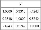
Notice that there is nothing random about the output from the VMTARGETCORR function. Randomness occurs only in step 4 of the algorithm.

You can obtain samples by calling the RANDVALEMAURELLI function, which returns an N × 3 matrix for this example, as follows:

/* generate samples from Vale-Maurelli distribution */ 
N = 10000;
call randseed(54321);
X = RandValeMaurelli(N, R, skew, kurt);

To verify that the simulated data in X have the specified properties, you can use PROC MEANS and PROC CORR to compute the sample moments and to visualize the multivariate distribution. The results are shown in Figure 16.18. Because estimates of the skewness and kurtosis are highly variable, 10,000 observations are used. However, to avoid overplotting only 1,000 observations are used to visualize the distribution of the simulated data, as follows:

create VM from X[c=(“x1”:“x3”)]; append from X; close VM;
quit;

proc means data=VM N Mean Var Skew Kurt;
run;

proc corr data=VM(obs=1000) noprob plots(maxpoints=NONE)=matrix(histogram);
ods select PearsonCorr MatrixPlot;
run;

Figure 16.18 Descriptive Statistics of Simulated Data

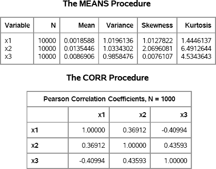
Figure 16.18 shows that the sample means are close to zero and the sample variances are close to unity. Taking into account sampling variation, the skewness and kurtosis are close to the specified values as are the correlations between variables.

Figure 16.19 shows the distribution of the simulated data. The Vale-Maurelli algorithm has generated nonnormal data with specified moments and with specified correlations.

Figure 16.19 Simulated Data by Using the Vale-Maurelli Algorithm

The Vale-Maurelli algorithm is simple to implement and usually works well in practice. Headrick and Sawilowsky (1999) note that the Vale-Maurelli algorithm can break down when the conditional distributions are highly skewed or heavy-tailed, and when the sample sizes are small. They propose an algorithm that is algebraically more complex but which seems to handle these more extreme situations.

16.12  References

Bowman, K. O. and Shenton, L. R. (1983), “Johnson's System of Distributions,” in S. Kotz, N. L. Johnson, and C. B. Read, eds., Encyclopedia of Statistical Sciences, volume 4, 303–314, New York: John Wiley & Sons.

Burr, I. W. (1942), “Cumulative Frequency Functions,” Annals of Mathematical Statistics, 13, 215–232.

Fan, X., Felsovályi, A., Sivo, S. A., and Keenan, S. C. (2002), SAS for Monte Carlo Studies: A Guide for Quantitative Researchers, Cary, NC: SAS Institute Inc.

Fleishman, A. (1978), “A Method for Simulating Non-normal Distributions,” Psychometrika, 43, 521–532.

Headrick, T. C. (2002), “Fast Fifth-Order Polynomial Transforms for Generating Univariate and Multivariate Nonnormal Distributions,” Computational Statistics and Data Analysis, 40, 685–711.

Headrick, T. C. (2010), Statistical Simulation: Power Method Polynomials and Other Transformations, Boca Raton, FL: Chapman & Hall/CRC.

Headrick, T. C. and Kowalchuk, R. K. (2007), “The Power Method Transformation: Its Probability Density Function, Distribution Function, and Its Further Use for Fitting Data,” Journal of Statistical Computation and Simulation, 77, 229–249.

Headrick, T. C. and Sawilowsky, S. (1999), “Simulating Correlated Multivariate Nonnormal Distributions: Extending the Fleishman Power Method,” Psychometrika, 64, 25–35.

Johnson, N. L. (1949), “Systems of Frequency Curves Generated by Methods of Translation,” Biometrika, 36, 149–176.

Johnson, N. L., Kotz, S., and Balakrishnan, N. (1994), Continuous Univariate Distributions, volume 1, 2nd Edition, New York: John Wiley & Sons.

Kendall, M. G. and Stuart, A. (1977), The Advanced Theory of Statistics, volume 1, 4th Edition, New York: Macmillan.

Ord, J. K. (2005), “Pearson System of Distributions,” in S. Kotz, N. Balakrishnan, C. B. Read, B. Vidakovic, and N. L. Johnson, eds., Encyclopedia of Statistical Sciences, volume 9, 2nd Edition, 6036–6040, New York: John Wiley & Sons.

Rodriguez, R. N. (2005), “Burr Distributions,” in S. Kotz, N. Balakrishnan, C. B. Read, B. Vidakovic, and N. L. Johnson, eds., Encyclopedia of Statistical Sciences, volume 1, 2nd Edition, 678–683, New York: John Wiley & Sons.

Slifker, J. F. and Shapiro, S. S. (1980), “The Johnson System: Selection and Parameter Estimation,” Technometrics, 22, 239–246.

Tadikamalla, P. (1980), “On Simulating Non-normal Distributions,” Psychometrika, 45, 273–279.

Vale, C. and Maurelli, V. (1983), “Simulating Multivariate Nonnormal Distributions,” Psychometrika, 48,465–471.

Vargo, E., Pasupathy, R., and Leemis, L. M. (2010), “Moment-Ratio Diagrams for Univariate Distributions,” Journal of Quality Technology, 42, 1–11.