The way Moore's Law has benefitted QlikView is really unprecedented amongst other BI systems.

QlikView began life in 1993 in Lund, Sweden. Originally titled "QuickView", they had to change things when they couldn't obtain a copyright on that name, and thus "QlikView" was born.

After years of steady growth, something really good happened for QlikView around 2005/2006—the Intel x64 processors became the dominant processors in Windows servers. QlikView had, for a few years, supported the Itanium version of Windows; however, Itanium never became a dominant server processor. Intel and AMD started shipping the x64 processors in 2004 and, by 2006, most servers sold came with an x64 processor—whether the customer wanted 64-bit or not. Because the x64 processors could support either x86 or x64 versions of Windows, the customer didn't even have to know. Even those customers who purchased the x64 version of Windows 2003 didn't really know this because all of their x86 software would run just as well (perhaps with a few tweaks).

But x64 Windows was fantastic for QlikView! Any x86 process is limited to a maximum of 2 GB of physical memory. While 2 GB is quite a lot of memory, it wasn't enough to hold the volume of data that a true enterprise-class BI tool needed to handle. In fact, up until version 9 of QlikView, there was an in-built limitation of about 2 billion rows (actually, 2 to the power of 31) in the number of records that QlikView could load. On x86 processors, QlikView was really confined to the desktop.

x64 was a very different story. Early Intel implementations of x64 could address up to 64 GB of memory. More recent implementations allow up to 256 TB, although Windows Server 2012 can only address 4 TB. Memory is suddenly less of an obstacle to enterprise data volumes.

The other change that happened with processors was the introduction of multi-core architecture. At the time, it was common for a high-end server to come with 2 or 4 processors. Manufacturers came up with a method of putting multiple processors, or cores, on one physical processor. Nowadays, it is not unusual to see a server with 32 cores. High-end servers can have many, many more.

One of QlikView's design features that benefitted from this was that their calculation engine is multithreaded. That means that many of QlikView's calculations will execute across all available processor cores. Unlike many other applications, if you add more cores to your QlikView server, you will, in general, add more performance.

So, when it comes to looking at performance and scalability, very often, the first thing that people look at to improve things is to replace the hardware. This is valid of course! QlikView will almost always work better with newer, faster hardware. But before you go ripping out your racks, you should have a good idea of exactly what is going on with QlikView. Knowledge is power; it will help you tune your implementation to make the best use of the hardware that you already have in place.

The following are the topics we'll be covering in this chapter:

Reviewing basic performance tuning techniques

There are many ways in which you may have learned to develop with QlikView. Some of them may have talked about performance and some may not have. Typically, you start to think about performance at a later stage when users start complaining about slow results from a QlikView application or when your QlikView server is regularly crashing because your applications are too big.

In this section, we are going to quickly review some basic performance tuning techniques that you should, hopefully, already be aware of. Then, we will start looking at how we can advance your knowledge to master level.

Removing unneeded data

Removing unneeded data might seem easy in theory, but sometimes it is not so easy to implement—especially when you need to negotiate with the business. However, the quickest way to improve the performance of a QlikView application is to remove data from it. If you can reduce your number of fact rows by half, you will vastly improve performance. The different options are discussed in the next sections.

Reducing the number of rows

The first option is to simply reduce the number of rows. Here we are interested in Fact or Transaction table rows—the largest tables in your data model. Reducing the number of dimension table rows rarely produces a significant performance improvement.

The easiest way to reduce the number of these rows is usually to limit the table by a value such as the date. It is always valuable to ask the question, "Do we really need all the transactions for the last 10 years?" If you can reduce this, say to 2 years, then the performance will improve significantly.

We can also choose to rethink the grain of the data—to what level of detail we hold the information. By aggregating the data to a higher level, we will often vastly reduce the number of rows.

Reducing the number of columns

The second option is to reduce the width of tables—again, especially Fact or Transaction tables. This means looking at fields that might be in your data model but do not actually get used in the application. One excellent way of establishing this is to use the Document Analyzer tool by Rob Wunderlich to examine your application (http://robwunderlich.com/downloads).

As well as other excellent uses, Rob's tool looks at multiple areas of an application to establish whether fields are being used or not. It will give you an option to view fields that are not in use and has a useful DROP FIELD Statements listbox from which you can copy the possible values. The following screenshot shows an example (from the default document downloadable from Rob's website):

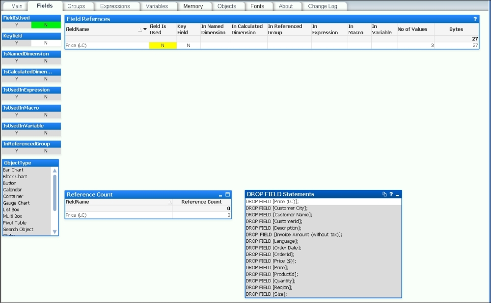
Adding these DROP FIELD statements into the end of a script makes it very easy to remove fields from your data model without having to dive into the middle of the script and try to remove them during the load—which could be painful.

There is a potential issue here; if you have users using collaboration objects—creating their own charts—then this tool will not detect that usage. However, if you use the DROP FIELD option, then it is straightforward to add a field back if a user complains that one of their charts is not working.

Of course, the best practice would be to take the pain and remove the fields from the script by either commenting them out or removing them completely from their load statements. This is more work, because you may break things and have to do additional debugging, but it will result in a better performing script.

Replacing text keys with numbers

Often, you will have a text value in a key field, for example, something like an account number that has alphanumeric characters. These are actually quite poor for performance compared to an integer value and should be replaced with numeric keys.

Note

There is some debate here about whether this makes a difference at all, but the effect is to do with the way the data is stored under the hood, which we will explore later. Generated numeric keys are stored slightly differently than text keys, which makes things work better.

The strategy is to leave the text value (account number) in the dimension table for use in display (if you need it!) and then use the AutoNumber function to generate a numeric value—also called a surrogate key—to associate the two tables.

For example, replace the following:

Account:
Load
   AccountId,
   AccountName,
   …
From Account.qvd (QVD);

Transaction:
Load
   TransactionId,
   AccountId,
   TransactionDate,
   …
From Transaction.qvd (QVD);

With the following:

Account:
Load
   AccountId,
   AutoNumber(AccountId) As Join_Account,
   AccountName,
   …
From Account.qvd (QVD);

Transaction:
Load
   TransactionId,
   AutoNumber(AccountId) As Join_Account,
   TransactionDate,
   …
From Transaction.qvd (QVD);

The AccountId field still exists in the Account table for display purposes, but the association is on the new numeric field, Join_Account.

We will see later that there is some more subtlety to this that we need to be aware of.

Resolving synthetic keys

A synthetic key, caused when tables are associated on two or more fields, actually results in a whole new data table of keys within the QlikView data model.

The following screenshot shows an example of a synthetic key using Internal Table View within Table Viewer in QlikView:

In general, it is recommended to remove synthetic keys from your data model by generating your own keys (for example, using AutoNumber):

Load
   AutoNumber(CountryID & '-' & CityID) As ClientID,
   Date,
   Sales
From Fact.qvd (qvd);

The following screenshot shows the same model with the synthetic key resolved using the AutoNumber method:

This removes additional data in the data tables (we'll cover more on this later in the chapter) and reduces the number of tables that queries have to traverse.

Reviewing the basics

So, with a basic understanding of QlikView development, you already have a good idea of how to improve performance. After reading the rest of this chapter, you will have enough information to seriously move forward and master this subject.