
"It is a capital mistake to theorize before one has data. Insensibly one begins to twist facts to suit theories, instead of theories to suit facts." | ||
| --Sherlock Holmes (Arthur Conan Doyle), A Scandal in Bohemia | ||
In data warehousing and business intelligence, there are many approaches to data modeling. We hear of personalities such as Bill Inmon and Ralph Kimball. We talk of normalization and dimensional modeling. But we also might have heard about how QlikView can cut across all of this—we don't need to worry about data warehousing; we just load in all the data from source systems and start clicking. Right?
Well, that might be right if you want to load just a very quick application directly from the data source and aren't too worried about performance or maintainability. However, the dynamic nature of the QlikView script does not mean that we should throw out all of the best practices in data warehouse design that have been established over the course of many years.
In this chapter, we are going to look at the best practices around QlikView data modeling. As revealed in the previous chapter, this does not always mean the best performing data model. But there are many reasons why we should use these best practices, and these will become clear over the course of this chapter and the next.
The following are the topics we'll be covering in this chapter:
- Reviewing basic data modeling
- Dimensional data modeling
- Handling slowly changing dimensions
- Dealing with multiple fact tables in one model
If you have attended QlikView training courses and done some work with QlikView modeling, there are a few things that you will know about, but I will review them just to be sure that we are all on the same page.
QlikView uses an associative model to connect data rather than a join model. A join model is the traditional approach to data queries. In the join model, you craft a SQL query across multiple tables in the database, telling the database management system (DBMS) how those tables should be joined—whether left, inner, outer, and so on. The DBMS might have a system in place to optimize the performance of those queries. Each query tends to be run in isolation, returning a result set that can be either further explored—Excel pivot tables are a common use case here—or used to build a final report. Queries might have parameters to enable different reports to be executed, but each execution is still in isolation. In fact, it is the approach that underlies many implementations of a "semantic layer" that many of the "stack" BI vendors implement in their products. Users are isolated from having to build the queries—they are built and executed by the BI system—but each query is still an isolated event.
In the associative model, all the fields in the data model have a logical association with every other field in the data model. This association means that when a user makes a selection, the inference engine can quickly resolve which values are still valid—possible values—and which values are excluded. The user can continue to make selections, clear selections, and make new selections, and the engine will continue to present the correct results from the logical inference of those selections. The user's queries tend to be more natural and it allows them to answer questions as they occur.
It is important to realize that just putting a traditional join model database into memory, as many vendors have started to do, will not deliver the same interactive associative experience to users. The user will probably get faster running queries, but they will still be isolated queries.
Saying that, however, just because QlikView has a great associative model technology, you still need to build the right data model to be able to give users the answers that they don't know and are looking for, even before they have asked for them!
We should know that QlikView will automatically associate two data tables based on both tables containing one or more fields that match exactly in both name and case. QlikView fields and table names are always case sensitive—Field1 does not match to FIELD1 or field1.
Suppose that we run a very simple load statement such as the following:
Customer:
Load * Inline [
CustomerID, Customer
1, Customer A
2, Customer B
];

Sales:
Load * Inline [
Date, CustomerID, Value
2014-05-12, 1, 100
2014-05-12, 2, 200
2014-05-12, 1, 100
];
This will result in an association that looks like the following:
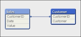
If you read the previous chapter, you will know that this will generate two data tables containing pointer indexes that point to several symbol tables for the data containing the unique values.
A synthetic key is QlikView's method of associating two tables that have more than one field in common. Before we discuss the merits of them, let's first understand exactly what is happening with them.
For example, consider the following simple piece of script:
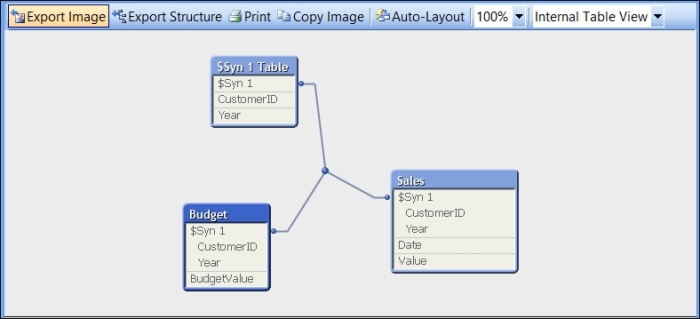
Budget:
Load * Inline [
CustomerID, Year, BudgetValue
1, 2013, 10000
2, 2013, 15000
1, 2014, 12000
2, 2014, 17500
];

Sales:
Load * Inline [
Date, Year, CustomerID, Value
2013-01-12, 2013, 1, 100
2013-02-25, 2013, 2, 200
2013-02-28, 2013, 1, 100
2013-04-04, 2013, 1, 100
2013-06-21, 2013, 2, 200
2013-08-02, 2013, 1, 100
2014-05-12, 2014, 1, 100
2014-05-12, 2014, 2, 200
2014-05-12, 2014, 1, 100
];
This will produce an Internal Table View like the following:
It is worth noting that QlikView can also represent this as a Source Table View, showing the association in a more logical, database way, like the following:

Note
To be honest, I never use this view, but I can understand why some people, especially those transitioning from a SQL background, might feel comfortable with it. I would urge you to get more comfortable with Internal Table View because it is more reflective of what is happening internally in QlikView.
We can see from Internal Table View that QlikView has moved the common fields into a new table, $Syn 1 Table, that contains all the valid combinations of the values. The values have been replaced in the original tables with a derived composite key, or surrogate key, that is associated with $Syn 1 Table.
To me, this is perfectly sensible data modeling. When we look at our options later on in the chapter, we will begin to recognize this approach as Link Table modeling. There are, however, some scare stories about using synthetic keys. In fact, in the documentation, it is recommended that you remove them. The following is quoted from QlikView Reference Manual:
When the number of composite keys increases, depending on data amounts, table structure and other factors, QlikView may or may not handle them gracefully. QlikView may end up using excessive amounts of time and/or memory. Unfortunately, the actual limitations are virtually impossible to predict, which leaves only trial and error as a practical method to determine them.
An overall analysis of the intended table structure by the application designer. is recommended, including the following:
Forming your own non-composite keys, typically using string concatenation inside an AutoNumber script function.
Making sure only the necessary fields connect. If, for example, a date is used as a key, make sure not to load e.g. year, month or day_of_month from more than one internal table.
The important thing to look at here is that it says, "When the number of composite keys increases…"—this is important because you should understand that a synthetic key is not necessarily a bad thing in itself. However, having too many of them is, to me, a sign of a poor data modeling effort. I would not, for example, like to see a table viewer looking like the following:

There have been some interesting discussions about this subject in the Qlik community. John Witherspoon, a long time contributor to the community, wrote a good piece entitled Should we stop worrying and love the Synthetic Key (http://community.qlik.com/thread/10279).
Of course, Henric Cronström has a good opinion on this subject as well, and has relayed it in Qlik Design Blog at http://community.qlik.com/blogs/qlikviewdesignblog/2013/04/16/synthetic-keys.
My opinion is similar to Henric's. I like to see any synthetic keys resolved in the data model. I find them a little untidy and a little bit lazy. However, there is no reason to spend many hours resolving them if you have better things to do and there are no issues in your document.
One of the methods used to resolve synthetic keys is to create your own composite key. A composite key is a field that is composed of several other field values. There are a number of ways of doing this, which we will examine in the next sections.
The very simplest way of creating a composite key is to simply concatenate all the values together using the & operator. If we were to revisit the previously used script and apply this, our script might now look like the following:
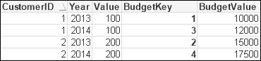
Budget:
Load
   CustomerID & Year as BudgetKey,
   BudgetValue
Inline [
CustomerID, Year, BudgetValue
1, 2013, 10000
2, 2013, 15000
1, 2014, 12000
2, 2014, 17500
];

Sales:
Load
   Date,
   Year,
   CustomerID,
   CustomerID & Year as BudgetKey,
   Value
Inline [
Date, Year, CustomerID, Value
2013-01-12, 2013, 1, 100
2013-02-25, 2013, 2, 200
2013-02-28, 2013, 1, 100
2013-04-04, 2013, 1, 100
2013-06-21, 2013, 2, 200
2013-08-02, 2013, 1, 100
2014-05-12, 2014, 1, 100
2014-05-12, 2014, 2, 200
2014-05-12, 2014, 1, 100
];
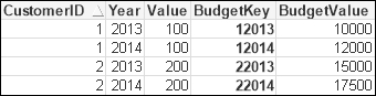
When we reload this code, the table viewer will look like the following screenshot:

The synthetic key no longer exists and everything looks a lot neater.
To see the composite key in action, I like to use a table box with values from both tables, just to see that the association works:
A table box works very well for this use case. I utilize them all the time when testing key associations like this. It is almost the only time that I use table boxes these days! In a normal user interface, a table box can be useful to display transaction-level information, but you can also use a straight table for this and have far more control with the chart than with the table. Totals, set analyses in expressions, and visual cues are all things that you can have in a straight table that you can't have in a table box.
We need to concern ourselves with key collision potentials; in this case, the key value of 12013, composed of the CustomerID value of 1 and the Year value of 2013. Let's imagine a further set of values where the CustomerID value is 120 and the Year value is 13. That would cause a problem because both combinations would be 12013. For that reason, and this should be considered a best practice, I would prefer to see an additional piece of text added between the two keys like the following:
   ...
   CustomerID & '-' & Year as BudgetKey,
   ...
If we do that, then the first set of values would give a key of 1-2013 and the second would give a key of 120-13—there would no longer be a concern about key collision. The text that you use as the separator can be anything—characters such as the hyphen, underscore, and vertical bar are all commonly used.
A Hash function takes the number of fields as a parameter and creates a fixed length string representing the hash of those values. The length of the string, and hence the possibility of having key collisions, is determined by the hash bit length. There are the following three functions:
Hash128()Hash160()Hash256()
The number at the end of the function name (128, 160, or 256) represents the number of bits that will be used for the hash string. We don't really need to worry too much about the potential for key collision—in his blog post on the subject, Barry Harmsen, co-author of QlikView 11 for Developers, Packt Publishing, worked out that the chance of a collision using Hash128() was one in 680 million (http://www.qlikfix.com/2014/03/11/hash-functions-collisions/).
Of course, if you do have a large dataset where that risk becomes greater, then using the Hash256() function instead will reduce the possibility to, effectively, zero. Of course, a longer hash key will take up more space.
If we were to use a Hash function in our script, it would look like the following:
Budget:
Load
   Hash128(CustomerID, Year) as BudgetKey,
   BudgetValue
   ...
Sales:
Load
   Date,
   Year,
   CustomerID,
   Hash128(CustomerID, Year) as BudgetKey,
   Value
   ...
Notice that the function just takes a list of field values. The Hash functions are deterministic—if you pass the same values to the function, you will get the same hash value returned. However, as well as having the same values, the order that the fields are passed in the function must also be identical.
This load will produce values that look like the following in my table box:
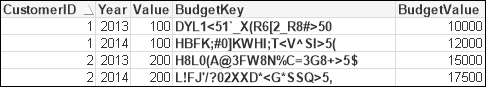
The other thing that is important to know about the Hash functions is that their deterministic nature should transcend different reloads on different machines. If you run the same script as I did, on the same version of QlikView, you should get the same result.
One of the problems with both of the two previously mentioned approaches is that the keys that are generated are string values and, as we saw in the previous chapter, they will take up a lot of space. It is far more efficient to use integer keys—and especially sequential integer keys (because they are not stored in the symbol tables). The AutoNumber function will do that for us.
The AutoNumber function will accept a string value and return an integer. How it works is that during the brief lifetime of a load script execution, QlikView maintains an internal database to store the passed string values. If you pass exactly the same value, then you will get exactly the same integer returned. It can be said to be deterministic (given the same input, you will get the same output), but only within the current execution of the script.
Note
This last point is important to note. If I pass "XXX" and get a return of 999 today, I cannot guarantee that "XXX" will return 999 tomorrow. The internal database is created anew at each execution of the script, and so the integer that is returned depends on the values that are passed during the load. It is quite likely that tomorrow's dataset will have different values in different orders so will return different integers.
AutoNumber will accept two possible parameters—a text value and an AutoID. This AutoID is a descriptor of what list of sequential integers will be used, so we can see that we have multiple internal databases, each with its own set of sequential integers. You should always use an AutoID with the AutoNumber function.
When creating a composite key, we combine the AutoNumber function with the string concatenation that we used previously.
If we modify our script to use AutoNumber, then it should look something like the following:
Budget:
Load
   Year, CustomerID,
   AutoNumber(CustomerID & '-' & Year, 'Budget') as BudgetKey,
   BudgetValue
   ...


Sales:
Load
   Date,
   Year,
   CustomerID,
   AutoNumber(CustomerID & '-' & Year, 'Budget') as BudgetKey,
   Value
   ...
The table box will look like the following:
We now have a sequential integer key instead of the text values.
One thing that is interesting to point out is that the string values for keys make it easy to see the lineage of a key—you can discern the different parts of the key. I will often keep the keys as strings during a development cycle just for this reason. Then, when moving to production, I will change them to use AutoNumber.
One thing that new QlikView developers, especially those with a SQL background, have difficulty grasping is that when QlikView performs a calculation, it performs it at the correct level for the table in which the fact exists. Now, I know what I just wrote might not make any sense, but let me illustrate it with an example.
If I have an OrderHeader table and an OrderLine table in SQL Server, I might load them into QlikView using the following script:
OrderHeader:
LOAD OrderID,
  OrderDate,
  CustomerID,
  EmployeeID,
  Freight;
SQL SELECT *
FROM QVTraining.dbo.OrderHeader;

OrderLine:
LOAD OrderID,
  "LineNo",
  ProductID,
  Quantity,
  SalesPrice,
  SalesCost,
  LineValue,
  LineCost;
SQL SELECT *
FROM QVTraining.dbo.OrderLine;
Note that there are facts here at different levels. In the OrderLine table, we have the LineValue and LineCost facts. In the OrderHeader table, we have the Freight fact.
If I want to look at the total sales and total freights by a customer, I could create a chart like the following:
Dimension | Total Freight Expression | Total Sales Expression |
|---|---|---|
|
|
|
This would produce a straight table that looks as follows:

Now, this is actually correct. The total freights and sales values are correctly stated for each customer. The values have been correctly calculated at the level that they exist in the data model.
If I were to do something similar in SQL, I might create a query like the following:
SELECT
   OH.CustomerID,
   CAST(Sum(OH.Freight) As money) As [Total Freight],
   CAST(SUM(OL.LineValue) As money) As [Total Sales]
FROM OrderHeader OH
INNER JOIN OrderLine OL
ON OH.OrderID=OL.OrderID
GROUP BY OH.CustomerID
ORDER BY 1
The result might look like the following screenshot:
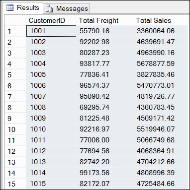
We can see that the sales values match with QlikView, but the freight values are totally overstated. This is because the freight values have been brought down a level and are being totaled with the same freight value repeated for every line in the one order. If the freight value was $10 for an order and there were 10 order lines, QlikView would report a correct freight value of $10 while the SQL query would give us an incorrect value of $100.
This is really important for us to know about when we come to data modeling. We need to be careful with this. In this instance, if a user were to drill into a particular product, the freight total will still be reported at $10. It is always worth checking with the business whether they need those facts to be moved down a level and apportioned based on a business rule.
As part of basic training, you should have been introduced to the concepts of join, concatenate, and ApplyMap. You may have also heard of functions such as Join and Keep. Hopefully, you have a good idea of what each does, but I feel that it is important to review them here so that we all know what is happening when we use these functions and what the advantages and disadvantages are of using the functions in different scenarios.
Even though the QlikView data model is an associative one, we can still use joins in the script to bring different tables together into one. This is something that you will do a lot when data modeling, so it is important to understand.
As with SQL, we can perform inner, left, right, and outer joins. We execute the joins in a logically similar way to SQL, except that instead of loading the multiple tables together in one statement, we load the data in two or more statements, separated by Join statements. I will explain this using some simple data examples.
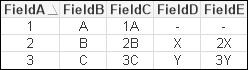
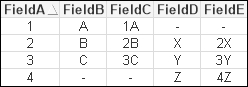
An inner join will join two tables together based on matches across common key values. If there are rows in either table where there are no matches, then those rows will no longer exist in the final combined table. The following is an example load:
Table1:
Load * Inline [
FieldA, FieldB, FieldC
1, A, 1A
2, B, 2B
3, C, 3C
];

Inner Join (Table1)
Load * Inline [
FieldA, FieldD, FieldE
2, X, 2X
3, Y, 3Y
4, Z, 4Z
];
This will result in a single table with five fields and two rows that looks like the following:

I describe an inner join as destructive because it will remove rows from either table. Because of this, you need to think carefully about its use.
I use left joins quite frequently, but rarely a right one. Which is which? Well, the first table that you load is the left table. The second table that you use the Join statement on is the right table.
The left join will keep all records in the left, or first, table and will join any matching rows from the right table. If there are rows in the right table that do not match, they will be discarded. The right join is the exact opposite. As such, these joins are also destructive as you can lose rows from one of the tables.
We will use the previous example script and change Inner to Left:
...
Left Join (Table1)
...
This results in a table that looks like the following:
Note that the first row has been retained from the left table, despite there being no matches. However, FieldD and FieldE in that row are null.
Changing from Left to Right will result in the following table:
In this case, the row from the left table has been discarded while the unmatched row from the right table is retained with null values.
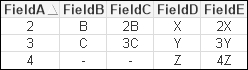
An outer join will retain all the rows from all the tables. Matching rows will have all their values populated whereas unmatched rows will have null values in the appropriate fields.
For example, if we replace the Left or Right join in the previous script with the word Outer, then we will get a table similar to the following:
For newbie QlikView developers who have come from the world of SQL, it can be a struggle to understand that you don't get to tell QlikView which fields it should be joining on. You will also notice that you don't need to tell QlikView anything about the datatypes of the joining fields.
This is because QlikView has a simple rule on the join—if you have fields with the same field names, just as with the associative logic, then these will be used to join. So you do have some control over this because you can rename fields in both tables as you are loading them.
The datatype issue is even easier to explain—QlikView essentially doesn't do datatypes. Most data in QlikView is represented by a dual—a combination of formatted text and a numeric value. If there is a number in the dual, then QlikView uses this to make the join—even if the format of the text is different.
But what happens if you don't have any fields to join on between the two tables? What we get in that scenario is a Cartesian join—the product of both tables. Let's have a look at an example:
Rene:
Load * Inline [
Field1, Field2
1, A
2, B
3, C
];
Join (Rene)
Load * Inline [
Field3, Field4
4, X
5, Y
6, Z
];
This results in a table like the following:
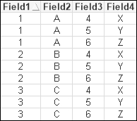
We can see that every row in the first table has been matched with each row in the second table.
Now this is something that you will have to watch out for because even with moderately sized datasets, a Cartesian join will cause a huge increase in the number of final rows. For example, having a Cartesian join between two tables with 100,000 rows each will result in a joined table with 10,000,000,000 rows! This issue quite often arises if you rename a field in one table and then forget to change the field in a joined table.
Saying that though, there are some circumstances where a Cartesian product is a desired result. There are some situations where I might want to have every value in one table matched with every value in another. An example of this might be where I match every account number that I have in the system with every date in the calendar so that I can calculate a daily balance, whether there were any transactions on that day or not.
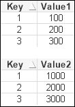
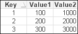
If you have some understanding of joins, you will be aware that when one of the tables has rows with duplicate values of the join key—which is common with primary to foreign key joins—then the resultant table will also have multiple rows. A quick example to illustrate this is as follows:
Dimension:
Load * Inline [
KeyField, DimensionValue
1, One
2, Two
3, Three
];

Left Join (Dimension)
Load * Inline [
KeyField, Value
1, 100
2, 200
3, 301
3, 302
];
This will result in a table like the following:

We have two rows for the KeyField value 3. This is expected. We do need to be careful though that this situation does not arise when joining data to a fact table. If we join additional tables to a fact table, and that generates additional rows in the fact table, then all of your calculations on those values can no longer be relied on as there are duplicates. This is definitely something that you need to be aware of when data modeling.
What if there are duplicate key values in both tables? For example, suppose that the first table looked like the following:
Dimension:
Load * Inline [
KeyField, DimensionValue
1, One
2, Two
3, Three.1
3, Three.2
3, Three.3
];
This will lead us to a table that looks like the following:
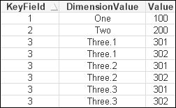
The resulting number of rows is the product of the number of keys in each table. This is something that I have seen happen in the field and something that you really need to look out for. The symptoms will be a far-longer-than-expected load time and large amounts of memory consumed. Have a look at this, perhaps silly, example:
BigSillyTable:
Load
   Floor(Rand()*5) As Key1,
   Rand()*1000 As Value1
Autogenerate(1000);

Join
Load
   Floor(Rand()*5) As Key1,
   Rand()*1000 As Value2
AutoGenerate(1000);
There are only 1,000 rows in each table with a low cardinality key that is duplicated (so there is an average of 200 rows per key). The resulting table will have approximately 200,000 rows!
This may seem a bit silly, but I have come across something similar.
The Keep syntax is quite interesting. It operates in a similar way to one of the destructive joins—it must take an inner, left, or right keyword—that means it will remove appropriate rows from the tables where there are no matches. However, it then leaves the tables as separate entities instead of joining them together into one.
As a use case, consider what might happen if you have a list of account numbers loaded and then used left Keep to load a transaction table. You would be left with the account and transaction tables as separate entities, but the transaction table would only contain rows where there was a matching row in the account table.
Concatenation in QlikView is quite similar to the Union All function in SQL (we can make it like a simple union by using the Distinct keyword when loading the tables). As with many things in QlikView, it is a little easier to implement than a union, in that you don't have to always ensure that both tables being concatenated have the same number of fields. If you concatenate tables with different numbers of fields, QlikView will go ahead and add any additional fields and populate nulls into any fields that didn't already have values. It is useful to review some of the aspects of Concatenate because we use it very often in data modeling.
If you have come across concatenation before, you should be aware that QlikView will automatically concatenate tables based on both tables having the exact same number of fields and having all fields with the same names (case sensitive). For example, consider the following load statements:
Table1:
Load * Inline [
A, B, C
1, 2, 3
4, 5, 6
];

Table2:
Load * Inline [
A, C, B
7, 8, 9
10, 11, 12
];
This will not actually end with two tables. Instead, we will have one table, Table1, with four rows:

If the two tables do not have identical fields, then we can force the concatenation to happen using the Concatenate keyword:
Table:
Load * Inline [
A, B, C
1, 2, 3
4, 5, 6
];

Concatenate (Table1)
Load * Inline [
A, C
7, 8
10, 11
];
This will result in a table like the following:

You will notice that the rows where there were no values for field B have been populated with null.
There is also a NoConcatenate keyword that might be useful for us to know about. It stops a table being concatenated, even if it has the same field names as an existing table. Several times, I have loaded a table in a script only to have it completely disappear. After several frustrating minutes debugging, I discovered that I have named the fields the same as an existing table—which causes automatic concatenation. My table hadn't really disappeared, the values had just been concatenated to the existing table.
Sometimes it can be difficult to understand what the effective difference is between Concatenate and Join and when we should use either of them. So, let's look at a couple of examples that will help us understand the differences.
Here are a couple of tables:
Now, if I load these tables with Concatenate, I will get a resulting table that looks like the following:

If I loaded this table with Join, the result looks like the following:
We will have a longer data table with Concatenate, but the symbol tables will be identical. In fact, the results when we come to use these values in a chart will actually be identical! All the QlikView functions that we use most of the time, such as Sum, Count, Avg, and so on, will ignore the null values, so we will get the same results using both datasets.
So, when we have a 1:1 match between tables like this, both Join and Concatenate will give us effectively the same result. However, if there is not a 1:1 match—where there are multiple key values in one or more of the tables—then Join will not produce the correct result, but Concatenate will. This is an important consideration when it comes to dealing with multiple fact tables, as we will see later.
This is one of my favorite functions in QlikView—I use it all the time. It is extremely versatile in moving data from one place to another and enriching or cleansing data. Let's review some of the functionality of this very useful tool.
The basic function of ApplyMap is to move data—usually text data—from a mapping table into a dimension table. This is a very normal operation in dimensional modeling. Transactional databases tend to be populated by a lot of mapping tables—tables that just have a key value and a text value.
The first thing that we need to have for ApplyMap is to load the mapping table of values to map from. There are a few rules for this table that we should know:
- A mapping table is loaded with a normal
Loadstatement that is preceded by aMappingstatement. - The mapping table can only have two columns.
- The names of the columns are not important—only the order that the columns are loaded is important:
- The first column is the mapping lookup value
- The second column is the mapping return value
- The mapping table does not survive past the end of the script. Once the script has loaded, all mapping tables are removed from memory.
- There is effectively no limit on the number of rows in the mapping table. I have used mapping tables with millions of rows.
- Mapping tables must be loaded in the script before they are called via
ApplyMap. This should be obvious, but I have seen some confusion around it.
As an example, consider the following table:
Mapping_Table:
Mapping
Load * Inline [
LookupID, LookupValue
1, First
2, Second
3, Third
];
There are a couple of things to note. First, let's look at the table alias—Mapping_Table. This will be used later in the ApplyMap function call (and we always need to explicitly name our mapping tables—this is, of course, best practice for all tables). The second thing to note is the names of the columns. I have just used a generic LookupID and LookupValue. These are not important. I don't expect them to associate to anything in my main data model. Even if they did accidentally have the same name as a field in my data model, there is no issue as the mapping table doesn't associate and doesn't survive the end of the script load anyway.
So, I am going to pass a value to the ApplyMap function—in this case, hopefully, either 1, 2, or 3—and expect to get back one of the text values—First, Second, or Third.
In the last sentence, I did say, "hopefully." This is another great thing about ApplyMap, in that we can handle situations where the passed ID value does not exist; we can specify a default value.
Let's look at an example of using the mentioned map:
Table:
Load
   ID,
   Name,
   ApplyMap('Mapping_Table', PositionID, 'Other') As Position
Inline [
ID, Name, PositionID
101, Joe, 1
102, Jane, 2
103, Tom, 3
104, Mika, 4
];
In the ApplyMap function, we have used the Mapping_Table table alias of our mapping table—note that we pass this value, in this case, as a string literal. We are passing the ID to be looked up from the data—PositionID—which will contain one of 1, 2, 3, or 4. Finally, we pass a third parameter (which is optional) to specify what the return value should be if there is no match on the IDs.
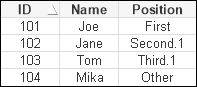
This load will result in the following table:

We can see that Joe, Jane, and Tom were successfully mapped to the correct position, whereas Mika, whose ID was 104, did not have a matching value in the mapping table so ended up with Other as the position value.
Something that many people don't think about, but which works very well, is to use the mapping functionality to move a number from one place to another. As an example, imagine that I had a product cost table in my database that stored the averaged cost for each product per month. I want to use this value in my fact table to calculate a margin amount per line. My mapping load may look something like the following:
Product_Cost_Map:
Mapping Load
   Floor(MonthStart(CostMonth)) & '-' & ProductID As LookupID,
   [Cost Value] As LookupValue;
SQL SELECT * From [Monthly Product Cost];
A good thing to note here is that we are using a composite key for the lookup ID. This is quite common and never an issue—as long as you use the exact same syntax and value types in the ApplyMap call.
Once we have this table loaded—and, depending on the database, this could have millions of rows—then we can use it in the fact table load. It will look something like this:
Fact:
Load
   ...
   SalesDate,
   ProductID,
   Quantity,
   ApplyMap('Product_Cost_Map', Floor(MonthStart(SalesDate)) & '-'
            & ProductID,0)
            *Quantity As LineCost,
   ...
In this case, we use the MonthStart function on the sales date and combine it with ProductID to create the composite key.
Here, we also use a default value of 0—if we can't locate the date and product combination in the mapping table, then we should use 0. We could, instead, use another mapping to get a default value:
Fact:
Load
   ...
   SalesDate,
   ProductID,
   Quantity,
   ApplyMap('Product_Cost_Map',
            Floor(MonthStart(SalesDate)) & '-' & ProductID,
            ApplyMap('Default_Cost_Map', ProductID, 0))
            *Quantity As LineCost,
   ...
So, we can see that we can nest ApplyMap calls to achieve the logic that we need.
We saw earlier in the discussion on joins that where there are rows with duplicate join IDs in one (or both) of the tables, the join will result in more rows in the joined table. This is often an undesired result—especially if you are joining a dimension value to a fact table. Creating additional rows in the fact table will result in incorrect results.
There are a number of ways of making sure that the dimension table that you join to the fact table will only have one row joined and not cause this problem. However, I often just use ApplyMap in this situation and make sure that the values that I want to be joined are sorted to the top. This is because in a mapping table, if there are duplicate key values, only the first row containing that key will be used.
As an example, I have modified the earlier basic example:
Mapping_Table:
Mapping
Load * Inline [
LookupID, LookupValue
1, First
2, Second.1
2, Second.2
3, Third.1
3, Third.2
3, Third.3
];
We can see that there are now duplicate values for the 2 and 3 keys. When we load the table as before, we will get this result:
We can see that the additional rows with the duplicate keys are completely ignored and only the first row containing the key is used. Therefore, if we make sure that the rows are loaded in the order that we want—by whatever order by clause we need to construct—we can just use ApplyMap to move the data into the fact table. We will be sure that no additional rows can possibly be created as they might be with Join.