
This is a bit of a recap recipe. In the workflow proposed here, we will sum up the tricks and knowledge gained throughout the book in order to perform a data-filtering activity.
Data filtering includes all the activities performed on a dataset to make it ready for further analysis.
Isn't it the same as data cleansing?
Well, in a sense… yes. However, not exactly the same, since data filtering usually refers to some specific techniques and not to others, while data cleansing can be considered a more comprehensive concept.
That said, here we will make tests for our data frame, performing subsequent filtering activities and reporting about these activities. The following diagram shows the flow:
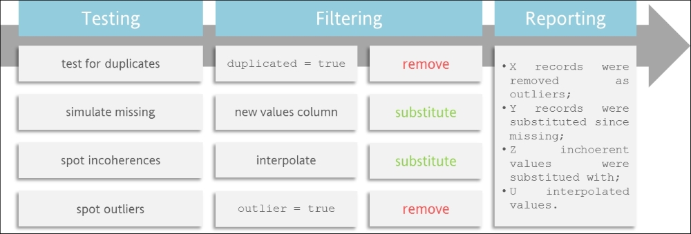
As you can see in the diagram, we will:
At the end of all these filtering activities, we will make our code produce a detailed report on the activities performed and results obtained.
The main value added here is to show how these activities can be performed as a unique workflow. This is actually quite common in real-life data analysis projects, where some tasks are preliminarily performed before we go on to the main activities.
To stress the point of the flow, I also suggest that you refer to the There's more... section to learn how to transform this flow within a custom function in order to let you apply it quickly every time you need it.
Before actually working on our data frame, we will create it here.
As mentioned earlier, we want to find outliers, incoherences, missing values, and duplicates. So, let's create a really bad data frame containing all these problems.
First, we will create a good dataset with data related to payments received from a customer:
dataset <- data.frame(
  key        = seq (1:251),
  date       = seq(as.Date("2012/5/12"), as.Date("2013/1/17"), by = "day"),
  attributes = c(rep("cash",times = 110),rep("transfer", times = 141)),
  value      = rnorm(251, mean = 100)
)
Our data frame will now have:
- A key column from 1 to 251.
- A date column with dates from May 12, 2012 to January 17, 2013.
- An attribute showing the kind of payment received, either cash or bank transfer.
- A value column, with values taken from a normal distribution with mean 100 (I used normal distribution just because it is cool, but data distribution is absolutely irrelevant here). Now that we have got a healthy data frame, it is time to make it sick.
Let's start mixing payment types, just to be more realistic:
for (i in 1:120) {
  dataset[round(runif(1, 1,251)),3] <- dataset[round(runif(1, 1,251)),3]
}
Here, we will take a value from a randomly selected cell of the attributes column and put it into another randomly selected cell within the attributes column. We will do this 120 times with a for loop.
We will use runif() to select a first random number to use as the row index (we ask for a number between 1 and 251, the number of total rows). The value corresponding to the randomly selected row within the attributes column is then assigned to another randomly selected row within the attributes column.
Keep this process in mind, since we will use it again within a few lines.
Now, it is time to duplicate some values:
for (i in 1:20) {
  dataset[round(runif(1, 1,251)),] <- dataset[round(runif(1, 1,251)),]
}
We randomly copied (select) a row and pasted it into another row, overwriting the old one.
Time to make some outliers:
for (i in 1:3) {
  index <- round(runif(1, 1,251))
  dataset[index,4] <- dataset[index,4]*1.3
}
What are outliers? Values outside the crowd. So, we took a member of the crowd and multiplied it 1.3 times. Is that arbitrary? Yes it is, but from the Detecting and removing outliers recipe, you should know that even outlier detection is in some way arbitrary.
To create incoherences, which we will remove later, we just have to copy a date attribute and paste it randomly. This will produce more than one value for the same date:
for (i in 1:15) {
  dataset[round(runif(1, 1,251)),2] <- dataset[round(runif(1, 1,251)),2]
}
Creating missing values is the simplest task. You just need to take some random rows and set the value attribute for that row to NA:
for (i in 1:10) {
  dataset[round(runif(1, 1,251)),4] <- NA
}
It is now time to install and load the required packages:
install.packages("mice","dplyr")
library(mice)
library(dplyr)- Store the number of rows within the original dataset:
n_of_initial_records <- nrow(dataset)
- Compute the number of duplicates and store it:
n_duplicates <- sum(duplicated(dataset))
- Detect duplicated rows and delete them:
dataset <- distinct(dataset)
- Store the number of NAs:
n_na <- nrow(subset(dataset,is.na(dataset$value)))
- Simulate possible values for missing values and substitute them:
simulation_data   <- mice(dataset[,-2], method = "pmm")
simulated_data    <- complete(simulation_data)
dataset$simulated <- simulated_data$value
- Sort the dataset by date (or alternative key to spot incoherences):
dataset <- dataset[order(dataset$date),]
- Count the number of values for each date and store repeated dates with their frequency in the data frame:
dates_frequency <- table(dataset$date) dates_count <- data.frame(dates_frequency) colnames(dates_count) <- c("date","frequency") dates_repeated_count <- subset(dates_count,dates_count$frequency > 1) - Create a vector with repeated dates:
dates_repeated_list <- as.Date(as.character(dates_repeated_count$date))
- Define the number of interpolated data (where the number of repeated dates is equal to the number of interpolated values):
n_of_interpolated <- nrow(dates_repeated_count)
- Define the number of records removed because of incoherences:
n_of_removed_for_interpolation <- sum(dates_repeated_count$frequency)
- Interpolate values by computing the average of the previous and subsequent values:
for (i in 1:length(dates_repeated_list)) { i = 1 date_match_index <- match(dates_repeated_list[i],dataset$date) number_of_repeat <- dates_repeated_count[i,2] # find value for 1 day before and one day after, handling hypotesis of the first or the last value # in dataset being incoherent if(date_match_index == 1 | date_match_index == nrow(dataset)) { value_before = mean(dataset$simulated) value_after = mean(dataset$simulated) } else { value_before <- dataset$value[date_match_index-1] value_after <- dataset$value[date_match_index+number_of_repeat+1] } } # compute average interpolated_value <- mean(c(value_after,value_before)) # create a a new row with same date and average value interpolated_record <- data.frame(dataset[date_match_index,1:4],"simulated" =interpolated_value) # add interpolated record to general dataset dataset <- rbind(dataset,interpolated_record) # remove incoherencies dataset <- dataset[-(date_match_index:date_match_index+number_of_repeat),] } - Spot and remove outliers by storing the number of removed rows:
dataset_quantiles <- quantile(dataset$simulated, probs = c(0.25,0.75))
range <- 1.5 * IQR(dataset$simulated)
n_outliers <- nrow(subset(dataset, dataset$simulated < (dataset_quantiles[1] - range) | dataset$simulated > (dataset_quantiles[2] + range)) )
dataset <- subset(dataset, dataset$simulated >= (dataset_quantiles[1] - range) & dataset$simulated <= (dataset_quantiles[2] + range))
- Build a filtering activity report:
filtering_report <- paste0("FILTERING ACTIVITIES REPORT: - ", n_outliers, " records were removed as outliers; - ", n_na," records were substituted since missing; - ", n_of_removed_for_interpolation," inchoerent values were substitued with; - ", n_of_interpolated, " interpolated values. "," ", n_of_initial_records, " original records ", " (-) ", n_outliers+n_of_removed_for_interpolation," removed ", " (+) ", n_of_interpolated, " added ", " = ", nrow(dataset), " total records for filtered dataset") - Visualize your report:
message (filtering_report)
In step 1, we store the number of rows within the original dataset. This step is required to provide a detailed report about the activities performed at the end of the process. We count the number of rows in the original dataset by running nrow() on the dataset.
In step 2, we compute the number of duplicates and store it. How would you compute the number of duplicated rows?
We use the duplicated() function from base R. Running this function on the dataset results in a vector with the value True for every duplicated record and False for unique values.
We then sum up this vector, obtaining the number of duplicated rows.
We store the result of this basic computation in a variable to be employed later, in the reporting phase.
In step 3, we detect duplicated rows and delete them. In this step, we apply the distinct() function from the dplyr package. This function removes duplicated values within a data frame, leaving only unique records.
You may find it interesting to know that this function offers the ability to look not only for entirely duplicated rows, but also for duplicated values. This can be done by specifying the attribute against which you want to look for duplicates.
Let's have a look at this basic example to understand how:
data <- data.frame("alfa"= c("a","b","b", "b"), "beta" = c(1,2,4,4))As you can see, this data frame contains three duplicated values on column alfa and two completely duplicated values, the last two.
Let' try to remove the last two rows by running distinct() on the whole dataset:
This will result in the following dataset:

But what if we run distinct, specifying we want to look for duplicates only within the alfa column?
distinct(data,alfa)
This will result in the following print:

Here we are. We filtered the dataset only for rows where the alfa attribute is duplicated.
In step 4, we store the number of NAs. We skip to missing value handling. First, we store the number of missing values, counting the number of rows in a dataset resulted from a subset of the original one.
We filtered the dataset object in order to keep only missing values, using the is.na() function of base R. The number of rows in this dataset will be exactly the number of missing values within the original dataset.
In step 5, we simulate possible values for missing values and substitute them. This step leverages missing value handling techniques learned in the Substituting missing values using the mice package recipe introduced previously. You can find more details on its rationales and results in that recipe.
All we have to specify here is that after running this piece of code, we will have a new column within our dataset, a new column with no missing values. This column will be used as the value column.
In step 6, we sort the dataset by date (or alternative key to spot incoherences). This step starts the treatment of incoherences. It is actually a soft start, since we just order by date. Nevertheless, let me explain this briefly.
What we want to find out now is the presence of more records for a given attribute. In our example, we are assuming that the attribute is the day. We are therefore stating that if more than one payment was recorded for a unique day, an error must have occurred within the recording process, and we are going to treat these records as incoherent.
You can see that the date is only an example, since the key could be any kind of attribute, or even more than one attribute.
For instance, we could impose a constraint of this type:
- If more than one payment was recorded for a customer (first key) within a single day (second key), something must have occurred.
What is the bottom line here? Sort by your relevant attribute, not necessarily by the date.
In step 7, we count the number of values for each date and store in a data frame repeated dates, with their frequencies.
It is now time to find incoherent records. First, we will find them by counting how many times each date is recorded within the dataset.
This can be done by leveraging the table() function from base R. This function computes a frequency table for a given attribute within a dataset.
The resulting dates_frequency object will have the following shape:
Var1          Freq
2012-05-12    1
2012-05-13    1
2012-05-12    2
Given the explanation in the previous step, which of these lines underline incoherences? Those where Freq is greater than 1, since these cases show that more than one value was recorded for the same date.
That is why we create dates_repeated_count, a data frame containing only dates with a frequency greater than 1.
In step 8, we create a vector with repeated dates. This is quite a tricky step. To understand it, we need to think about the class of the date column in the date repeated_count.
Here is how we can do it.
We can run the str() function on it to understand which class is assigned to the date column:
> str(dates_repeated_count)
'data.frame': 13 obs. of  2 variables:
$ date     : Factor w/ 219 levels "2012-05-12","2012-05-13",..: 10 22 29 107 119 126 128 145 148 153 ...
 $ frequency: int  2 2 2 2 2 2 2 2 2 2 …
As you see, date is a Factor with 219 values, one for each unique date. Generally speaking, the Factor class is a really convenient class to handle categorical variables. In our case, we will need to transform it into a Date class.
Why? Because the column we will compare it with was defined as a Date column!
Casting is done using these two steps:
- First, we change the format from factor to character using the
as.character()function - Then, we transform the character function in the data using the
as.date()function
At the end of the process, we will have a new vector of class Date that stores only dates for which some incoherence was underlined.
In step 9, we define the number of interpolated data (where the number of repeated dates = the number of interpolated values). This step is within the family of accounting steps already performed. We just compute and store the number of interpolated values. How do we compute them? We just have to compute the number of repeated dates, since we will define an interpolated value for each incoherence.
This is exactly what we do when we count the number of rows within the dates_repeated_count.
In step 10, we define the number of records removed because of incoherences. Here, we want to understand and memorize how many records will be removed because they come, we assume, from errors within the recording process.
This number will equal the sum of the Freq column within the dataset that stores all repeated dates. Why?
Because the number of times a duplicated date is recorded within the original dataset is equal to the number of incoherent records for that date. Therefore, the sum of the number of times all duplicated dates are recorded within the original dataset will equal the total number of incoherences and therefore equal the number of records removed because they were incoherent.
It's a bit of a devious trip I know, but I am sure you have followed me.
In step 11, we interpolate values by computing the average of the previous and subsequent values. This is the actual core part of our treatment of incoherences.
In this step, we looped through all the dates where incoherences were found, which are stored within the previously defined dates_repeated_list. We defined an interpolated value for each of these dates.
Our interpolation approach is as follows:
- We look for the record before the duplicated date and store it within the
value_beforeobject - We look for the record after the duplicated date and store it within the
value_afterobject - We compute the mean of these two values
Here is a graphical explanation of this approach:

As you can see, we do not consider incoherent values and actually remove them from the dataset. Be aware that two special cases are handled in a quite different way. If incoherences are within the first or the last date, we simply interpolate using the mean of the overall value vector.
In step 12, we spot and remove outliers by storing the number of removed rows. Removing outliers was a task we performed in the Detecting and removing outliers recipe. Refer to this recipe to understand how we do this.
We need to ensure that the number of outliers removed is stored within the n_outliers variable.
In step 13, we build a filtering activity report. I have to admit this is one of my favorite parts. We sum up all the stored numbers by composing a detailed report on the activities performed and their results.
To accomplish this task, we created a vector by pasting together strings and numbers stored within the entire analysis.
I would like to highlight the use of the
token to start a new paragraph.
In step 14, we visualize the report. Running the (filtering_report) message will make your report appear on your console. As you can see, on reading the report, we can understand the impact of each activity performed and reconcile the original number of rows with the final one. This is a really useful feature, particularly when sharing the results of your activities with colleagues or external validators.