As mentioned earlier, Markdown is a popular markup language developed by John Gruber.
This language is based on the principle of the supremacy of plain text documents over all other kinds of format.
Plain text is the base for any subsequent kind of manipulation and will be always readable without any particular software. This will let your work be usable and understandable for years to come and will not let you become the hostage of a particular software provider.
Rmarkdown integrates the Markdown language with some facilities for R code integration, which lets you show results from running R code, such as plots or tables, in a Markdown document.
Let’s warm up by installing and loading the required packages:
install.packages(“rmarkdown”)
install.packages(“knitr")
library(rmarkdown)
library(knitr)
- Create a new R Markdown document:

- Remove the default content from the document, except for YAML parameters, as we don’t want to be bound by the already available default content. Just go and delete it. The only part I ask you to preserve is the first chunk of text enclosed within two ‘---’ tokens.
- Specify the YAML parameters to obtain the table of contents.
To add the table of contents, you have to remove this line:
output: html_documentInsert at the same point the following lines:
output:
 html_document:
  toc: yes
You should be aware that YAML is in some way “space sensitive." This means that the number of indentation spaces will be considered during document file rendering to understand the meaning of the full line of code.
In our example, we have to place one space before
html_documentand two spaces beforetoc: yes. The first space will let us readhtml_documentas a value of theoutputparameter, while the two spaces beforetoc: yeswill signify that this token is a value of thehtml_document:argument. - Add a setup chunk:
```{r setup, include=FALSE}
knitr::opts_chunk$set(echo = TRUE)
library(knitr)
```
- Add a main title:
#main title - Add a structure:
## first paragraph

## second paragraph

## first subparagraph
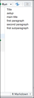
- Navigate the document structure using the outline viewer:
- Add a plot:
```{r plot, echo= FALSE}
plot(iris$Sepal.Length,iris$Petal.Width)
```
- Add a table from a dataset:
```{r kable, echo= FALSE}
kable(iris[1:10,])
```
- Give the possibility to fold the code.
Add the following to the
yamlparameters:code_folding: hide - Add a value within the text from the
relaboration.In an R Markdown document, it is also possible to expose a value that comes from running some R code. In our example, we will embed the number of rows composing the
irisdataset (150, if you are wondering). Two mandatory parts for embedding R output within a document are the`rtoken at the beginning and the`token at the end.`r nrow(iris)` - Add a link to external resources:
[link to the R project website](https://www.r-project.org) - Add a link to internal resources:
[link to chapter 7 codefile](chapter_7.R) - Embed a picture:
 - Render your document.
You can render you document through the knit control on the upper bar, or simply use Ctrl + Shift + K.
In step 1, the R Markdown is perfectly integrated in the RStudio environment. Creating a new R Markdown report just requires you to select the File menu and the New R Markdown report option.
In step 2, we just require you to delete the default content of the document. There is not much to say here, am I right?
In step 3, the yaml parameters are used during the rendering phase (which you will start in the last step of this recipe) to set some attributes of the document.
With an acceptable approximation, we can say that within the yaml chunk, we set the document’s metadata.
Adding a table of contents requires you to modify the output:html_document statement to let it receive more arguments to render the output.
Be aware that other parameters can be set for the HTML document. You can set them from the output options, which you can access in the following menu:

It’s even possible to specify a different kind of output from HTML, directly from the knit menu:

Refer to the Writing and styling PDF documents with RStudio recipe for more details on PDF outputs.lòk.
In step 4, the question to ask is, "What is a setup chunk?" I am sure you are guessing right. A setup chunk is a chunk of R code used to define the general settings of your document.
It is in no way different from other chunks, but it is a best practice to have all preliminary activities necessary for your analysis development in one place.
For instance you can place within this chunk package installation and loading, data frame import, code loading, and so on.
In step 5, we add a main title. This step and the following one will let you add a structure to your document, dividing it into paragraphs and subparagraphs, all starting with a principal title.
If you have some familiarity with HTML code, it will help you in the following table, which relates the HTML headers’ node tokens to the corresponding R Markdown code:
|
Html node |
R Markdown |
Output |
|---|---|---|
|
|
|
|
|
|
|
|
|
|
|
|
|
|
|
|
|
|
|
|
|
|
|
|
Adding a number for # greater than six will simply result in the # tokens not being shown and the following text being reproduced as body text.
In step 6, you can define a structure for your document using the heading shown in the previous step.
In step 7, among the features introduced with the 0.99 version, which deserves a place of honor, is certainly the outline viewer for R Markdown documents.
This viewer produces a navigable index for your document, letting you quickly understand the structure it is assuming.
To achieve this, the RStudio IDE looks for the previously introduced # tokens and for chunks of R code.
In step 8 we add a plot. The core feature of R Markdown is embedding embeds the results from an R environment within a markdown document.
- Even if our example here is a really basic one, it lets you completely understand the power of this feature
You can embed the results of R code computations, such as plots or tables, within your documents surrounding the piece of R code we want to run with the following tokens:
```{r name_of_the_chunck}
```
You can now decide some parameters to fine-tune the appearance of elaboration results. The ones you will more likely use are as follows:
Echo FALSE/TRUEspecifies whether results from the elaboration, different from plots, should be shown within the document.Warnings FALSE/TRUEshould be set totrueif you want R warnings to be printed out (for instance, warnings on package loading).Fig.captionis the caption of your plot, which sets the caption to be shown under plots (if any) produced from the chunk of code. Be aware of settingfig_caption = TRUEunderhtml_documentwithinyamlparameters to make captions visible. See step 3 for more information onyamlparameters.
You can get a sense of all the available settings by writing:
```{r name_of_chunk,
After inputting “,” RStudio will show you a list of possible settings.
You can find a complete and explained list of possible settings on the website of yihui xie, the author and maintainer of the knitr package, which is the base of the rmarkdown package. You can find the website at http://yihui.name/knitr/options/.
In step 9, we add a table from a dataset. One of the most annoying things in markdown is probably table creation. You have to input them cell by cell, dividing your cells by “|”.
Fortunately, R Markdown doesn’t require you to do this, but rather provides a really easy and convenient way of showing your data frames as well as formatted tables, simply by calling the kable() function.
In step 10, we provide the ability to fold the code. To let a code fold/unfold, the controls appear in the upper-right corner of your document. You can add the following parameter within the yaml section:
code_folding: hide
This will make the following control appear:

Using this control, the reader will be able to specify whether pieces of code will be shown within the document or not. This control can significantly enhance the readability of your document, especially if long chunks of code are introduced within the text.
In step 11, we add a value within the text that comes from from R elaboration. This is a really nice feature of R Markdown. It greatly broadens its horizons. Be aware that even those small scripts will have access to the general document environment and will therefore be able to use all objects and functions within this environment.
In step 12, we add a link to external resources. Including a link to external sources is useful, especially when writing documents to be published online. You can add an external link specifying a proper label (the text that will appear) within squared brackets and the actual link to point to between round brackets. Here is an example:
[text to show](“www.the_actual_url.com”)
In step 13, we add a link to internal resources. The main difference between this step and the previous one is the relative location of the linked file. In this case, we are pointing to a file placed in the working directory of the calling file (our R Markdown document). We can therefore just specify the piece of path from the directory we are working on.
In step 14, we embed a picture. With a script not too different from the one used for links, we can embed an image, specifying the location of the image file in round brackets.
In step 15 we render the document. If everything went right, after hitting the knit document button, you will see a new tab appear next to the console tab. The new tab will be labeled R Markdown.
In this new tab, logs from R Markdown processing will appear, acknowledging the activities being performed by RStudio to create an HTML file from your R Markdown document.
At the end of the process, your HTML document will show up.
Markdown is a really popular and always growing language.
You can use it in an increasing number of virtual places, from GitHub to Wordpress.
Here are some useful resources you can explore to broaden your topic knowledge:
- R Markdown official website for RStudio at http://rmarkdown.rstudio.com
- Markdown syntax introduction on the official markdown website at https://daringfireball.net/projects/markdown/syntax