
The linkcomm package is an R package developed with the main aim of letting you discover and study communities that exist within your network. These communities are discovered by applying an algorithm derived from the paper Link communities reveal multiscale complexity in networks by Ahn Y.Y., Bagrow J.P., and Lehmann.
In order to use linkcomm functionalities, we first need to install and load the linkcomm package:
install.packages("linkcomm")
library(linkcomm)
As a sample dataset, we will use the lesmiserables hedge list, provided in the linkcomm package. This dataset basically shows relations hips between characters in Victor Hugo's novel Les Misérables.
You can get a sense of the dataset by running str() on it:
> str(lesmiserables)
'data.frame':  254 obs. of  2 variables:
 $ V1: Factor w/ 73 levels "Anzelma","Babet",..: 61 49 55 55 21 33 12 23 20 62 ...
$ V2: Factor w/ 49 levels "Babet","Bahorel",..: 42 42 42 36 42 42 42 42 42 42 ...
- Create a
linkcommobject:linkcomm_object <- getLinkCommunities(lesmiserables, hcmethod = "single")

- Show network with communities:
plot(linkcom_obj, type = "graph", layout = layout.fruchterman.reingold)

- Select the nodes to be displayed:
plot(linkcom_obj, type = "graph", layout = "spencer.circle", shownodesin = 3)

- Show the composition of the communities:
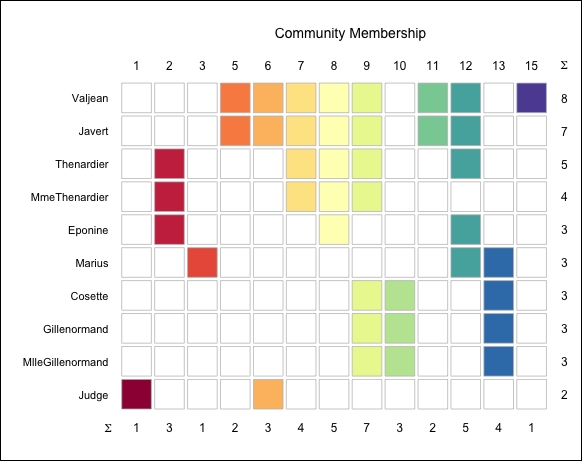
plot(linkcom_obj, type = "members")
This plot shows members and the community that they belong to:
In step 1, we create a linkcomm object. The linkcomm objects are, as you have probably guessed, the base components of every network visualization within the linkcomm package. These objects are characterized as a list object, storing relevant attributes for the given network.
It is interesting to note that linkcomm objects are built on the base of an igraph object, confirming the relevance of the latter package for network visualization in R.
What linkcomm adds to the igraph object is information about communities that exist within the network. These communities are derived by applying the cited algorithm on the hedge list provided. This is a good example of how the R community is able into begin the language development starting from what of good has already been done.
This algorithm basically looks for nodes that have a good enough number of common links and can be considered as clustering algorithms, as made clear by the dendogram that appears once getLinkCommunities() is executed.
In step 2, we show the network with communities. This step once again makes use of the plot() function's flexibility. As seen in the Looking at your data using the plot() function recipe, this function is able to change its output depending on the class of the data given as input. Refer to cited recipe for further information on this function.
Also note that it is possible to change the layout of your plot by modifying the layout argument in the plot() function.
Here are the available layouts:
spencer.circlelayout.randomlayout.circlelayout.spherelayout.fruchterman.reingoldlayout.kamada.kawailayout.springlayout.reingold.tilfordlayout.fruchterman.reingold.gridlayout.lgllayout.graphoptlayout.mdslayout.svdlayout.norm
Next, in step 3 we select the nodes to be displayed. When working with large networks, having the possibility to focus your attention on just a selection of them is a really useful feature. The linkcomm package implements this feature through the shownodesin argument in the plot function. This parameter lets you virtually filter your nodes, highlighting only nodes pertaining to at least n communities, where n is a custom number having as a maximum the total number of identified communities.
Lastly, in step 4 we show the composition of the communities. The plot displayed in step 4 is a really useful visualization of our network, since it lets you easily analyze the composition of the communities. I hope that looking at these Les Misérables. character links will make you willing to read the great novel by Victor Hugo, or at least watch the movie!