Chapter 6

Compression of Physiological Signals

6.1. Introduction

The aim of this chapter is to provide the reader with a general overview of the compression of physiological signals. The specificities of these signals have been covered in Chapter 3; whereas, in this chapter, the EEG compression is discussed and special attention will be given to the ECG signal. This is explained by the fact that the ECG is somehow, more concerned with compression, especially when used for monitoring purposes. Moreover, a huge number of research publications are dedicated to the compression of this type of signal. In fact, some specific and various requirements, i.e. transmission by Internet, wireless transmission, long-term storage on Holter monitors (i.e. for 24 hours or more), make the compression of the ECG an important tool.

For the reasons outlined above, this chapter is organized as follows: in section 6.2, the main standards used for coding the physiological signals are presented. Section 6.3 is dedicated to EEG compression, while in section 6.4, various ECG compression techniques are described.

6.2. Standards for coding physiological signals

Unlike the DICOM standard, devoted to medical images, as discussed in Chapter 4, it is important to specify that an exclusive norm or standard does not exist for coding physiological signals. In other words, the few available norms are not systematically accepted by both the European and American communities. Nevertheless, it seems to us to be essential to look at the main existing norms, which are summarized below.

6.2.1. CEN/ENV 1064 Norm

This European standard, also known as “SCP-ECG”, has been specially developed to code the ECG. Using this norm, coding the signals can be achieved either in compressed mode or non-compressed mode [ENV 96]. It includes the information related to the sampling frequency, filtering as well as other useful specifications. This norm is usually suggested for use with ECG databases. it allows the user to share the same utility software for reading and analyzing the data.

6.2.2. ASTM 1467 Norm

This norm is mainly appropriate to neuro-physiological signals such as the electroencephalogram (EEG), evoked potentials (EP), electromyogram (EMG) [ASM 94]. It is also used for monitoring using ECG, gastrointestinal signal, etc. In addition, this norm specifically includes a set of useful clinical information such as:

– sampling frequency;

– channel identification;

– filter parameters;

– electrode positions;

– stimulation parameters;

– types of drugs used during the acquisition process, etc.

6.2.3. EDF norm

The EDF (European Data Format) norm was introduced in the last decade by a team of engineers actively working in the field of biomedical engineering [KEM 92]. The format which has been used allows an important flexibility for both exchange and storage of multichannel physiological signals. As in the previous norm, it includes clinical information related to both the patient and the acquisition protocol. This norm is commonly used in Europe and it was extended in 2002 with the proposed format EDF+.

6.2.4. Other norms

Finally, we can cite other norms such as the CEN-TC251/FEF [CEN 95], the EBS (extensible biosignal format) for EEGs and EMGs, the SIGIF for neurophysiological signals including the compression option, the MIT arrhythmia database format and finally the DICOM supplement 30, proposed by the DICOM committee following clinician recommendations.

The compression of physiological signals has not been systematically included in the codecs mentioned above. However, it seems obvious that the standardization of compression has now become an important target to be attained.

6.3. EEG compression

6.3.1. Time-domain EEG compression

Generally, most of the techniques proposed in the literature devoted to EEG compression are mainly prediction based. This can be explained by the fact that the EEG is a low-frequency signal, which is characterized by a high temporal correlation. Some of these techniques are in fact a direct application of classical digital signal processing methods. For instance, we can point out the Linear Prediction Coding (LPC), the Markovian Prediction, the Adaptive Linear Prediction and Neural Network Prediction based methods. On the other hand, some approaches include the information related to the long-term temporal correlation of the samples. In fact, if we analyze the correlation function of an EEG segment, we will note that spaced samples present a non-neglected correlation that should be taken into account during processing. This information might be integrated into various dedicated codecs. Finally, we can also evoke the techniques which consist of correcting the errors of the prediction using information intrinsic to the EEG. For more details, the reader can refer to the following reference [ANT 97].

6.3.2. Frequency-domain EEG compression

The compression of the EEG in the frequency domain did not come from classical techniques such as Karhunen-Loéve Transform (KLT) or the Discrete Cosine Transform (DCT). As has already been mentioned, the EEG signal is dominated by low frequencies, mainly lower than 20 Hz. in fact, it is considered that the main energy is located around the a rhythm (between 8 Hz and 13 Hz).

6.3.3. Time-frequency EEG compression

Among the time-frequency techniques, the wavelet transform has been commonly used to compress the EEG [CAR 04]. In this technique, the signal is segmented and decomposed using Wavelet Packets. The coefficients are coded afterwards. Other algorithms such as the well known EZW (Embedded Zerotree Wavelet) have also been successfully applied to compress the EEG signal [LU 04]. Even if the obtained results seem significant, we think that the various codecs can be improved by pre-processing the EEG signal by reducing or eliminating the artefacts, which contaminate the EEG.

6.3.4. Spatio-temporal compression of the EEG

These approaches have the advantage of combining two aspects. The first aspect consists of taking into consideration the temporal correlation using the techniques pointed out previously, whereas the second aspect includes the spatial correlation due to a multichannel record [ANT 97]. In this method, a lossless compression technique is used.

6.3.5. Compression of the EEG by parameter extraction

This last approach is different from the techniques introduced previously. In fact, the EEG is compressed using an uncommon method in the sense that only the main parameters which allow an objective diagnostic are extracted. They can either be stored or transmitted but cannot under any circumstances be used to reconstruct the temporal signal [AGA 01]. However, this approach involves three stages:

– segmentation: this consists of isolating the stationary EEG segment of interest;

– feature extraction: each EEG segment is modeled as a statistical process (AR, MA, ARMA, etc.);

– classification: the analysis of the extracted parameters allows the identification of the different phases of anomalies.

6.4. ECG compression

As pointed out in the introduction to this chapter, the EEG compression field has been somehow less critical than the ECG compression. However, in this section, some ECG compression techniques will be described. Some of them are appropriate for real time transmission, whereas others are more suitable for storage, basically when Holter monitors are used.

6.4.1. State of the art

For purposes of clarity, we have gathered in Table 6.1 the most recent research pertaining to the ECG compression field. This has been highlighted, on one hand by specifying the country of each concerned research team working in this field and on the other hand the corresponding methods used. In fact, if we consider the number of articles published over the past six years, we will observe that not less that 20 papers have been published in international journals. This clearly demonstrates the importance of this field of research.

The ECG compression techniques can be classified into three broad categories: direct methods, transform-based methods and parameter extraction methods. In the direct methods category, the original samples are compressed directly. In the transformation methods category, the original samples are transformed and the compression is performed in the new domain. Among the algorithms which employ the transforms, we can hold up several algorithms based on the discrete cosine transform, and the wavelet transform. In the category of the methods using the extraction of parameters, the features of the processed signal are extracted and then used a posteriori for the reconstruction.

In this chapter, the scheme (i.e. of three categories) presented above will not be taken as reference. In fact, this section is structured so that the ECG compression techniques dedicated to real time transmission are first presented in section 6.4.4, whereas in section 6.4.5, the techniques designed mainly for storage purpose are described. Both of these techniques will be preceded by two sections describing, on the one hand, the evaluation of the performances (section 6.4.2), and on the other hand, the pre-processing techniques of the ECG signal (see section 6.4.3).

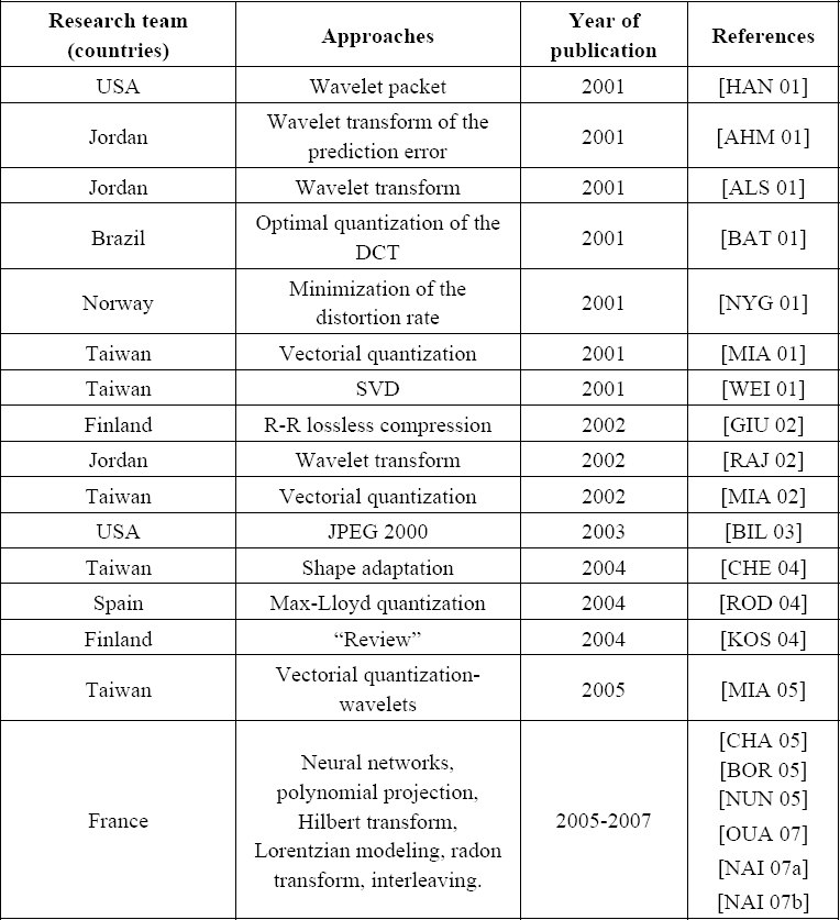
Table 6.1. Recent research work related to ECG compression

6.4.2. Evaluation of the performances of ECG compression methods

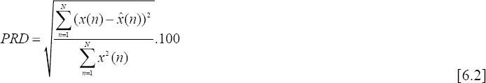
The performance of the proposed algorithm is evaluated using the Compression Ratio (CR) and the Percent Root-Mean-Square Difference (PRD) in % which is commonly used to measure the distortion resulting from ECG compression.

These two definitions are given by equations [6.1] and [6.2] respectively.

where:

N_x denotes the number of bits used to code the original signal;

denotes the number of bits used to code the reconstructed signal.

where:

x(n) is the original signal to be compressed, recorded on N samples;

(n) represents the reconstructed signal, recorded on N samples.

It is also important to point out that the PRD does not provide a significant evaluation, especially when the DC-component is included in the calculation; for more information, see [ALS 03]. In addition, even if the PRD and CR are considered as two important criteria for the evaluation of a given ECG compression technique, it is important to take into consideration other significant parameters, i.e. the calculation complexity for both coding and decoding as well as the robustness of the technique with respect to noise. In addition, we must specify whether the technique is more appropriate for real-time transmission or for storage.

6.4.3. ECG pre-processing

Based on the above comments, the first ECG pre-processing consists of suppressing the DC-component. This component can be added at the reception during the reconstruction process. A second important pre-processing technique consists of segmenting the ECG in order to isolate the different beats before the coding phase. In this case, the ECG signal is processed segment by segment. However, it is also important to know that if the segmentation is performed by a non-supervised approach, a border effect can be observed after the reconstruction phase.

Several ECG segmentation techniques have been studied in the literature for purposes of either compression or classification. The reader can refer for instance to various techniques using hidden Markov chains, wavelets [CLA 02] or genetic algorithms [GAC 03].

6.4.4. ECG compression for real-time transmission

In this section we present a certain number of techniques, classified according to their domain of processing, i.e. the time-domain or the frequency domain. These approaches are mainly based on parametrical modeling. The quantization and entropic coding will not be detailed in this chapter since these classical functionalities should be integrated into the final compression scheme. However, the time-domain approaches are described in section 6.4.4.1, while the frequency -domain approaches are presented in section 6.4.4.2.

6.4.4.1. Time domain ECG compression

6.4.4.1.1. Gaussian modeling of the ECG beat

If we consider x(1), x(2), ..., x(N), N samples of a measured ECG beat, denoted by x(n); modeling this signal using a sum of M Gaussians consists of approximating it by a set of Gaussians allowing the best fitting in the sense of least squares.

The model is defined as follows:

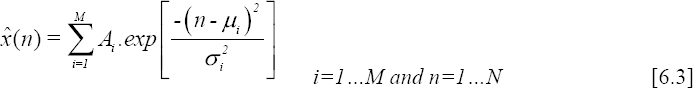
where A_i is the amplitude, μ_i (points along a temporal scale) is the mean value and σ_i is the standard deviation of Gaussian i.

Since, it is not evident to explicitly calculate the parameters of the model, this could be fitted using a non-linear least squares optimization technique.

It is clear that the choice of the Gaussian model is intuitive in the sense that the shape of each wave constituting a normal ECG beat can be approximated by a Gaussian. Therefore, in order to identify the parameters of equation 6.3, several optimization techniques can be used. For example, we can use any classical optimization technique suited to non-convex criteria, including the metaheuristic approaches. Of course, it is well known that these methods are time consuming, but if we consider that the ECG is a low frequency signal (i.e. one beat per second on average) and that the compression of the k^th beat is achieved during the acquisition of the (k+1)^th beat, the processing time generally becomes sufficient. In fact, some specific processors dedicated to Digital Signal Processing, like DSPs (Digital Signal Processors) or FPGAs (Field Programmable Gate Fields), can meet the real time requirements.

Let us reconsider our equation 6.3 for which we have to identify the parameters described above. These parameters can be determined simply by minimizing the following criterion:

This can also be expressed by:

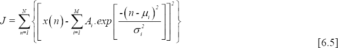
It is also evident that the number of Gaussians (M) to be used is of great importance. If M is under-estimated, the quality of the reconstructed signal decreases, whereas if the M is over estimated, the calculation increases. Thus, we can for example use some information criteria to identify the optimal order.

In practice, an empirical approach can be used to determine the most appropriate order. For example, experiences on normal and abnormal (for instance PVCs) beats show that an order of 5 or 6 can be suitable for modeling each ECG beat. It is also obvious that if the recorded ECG contains some specific significant high frequencies, we have to increase the order to fit the signal properly.

Figures 6.1 and 6.2 represent two typical ECG beats (normal/PVC) as well as their corresponding parametrical models. The PVC beat is reconstructed using 5 Gaussians, whereas the normal ECG beat is obtained using 6 Gaussians.

Using these approaches, the compression ratio depends of course on the following parameters:

– M: number of Gaussians (model order) used to reconstruct an ECG beat;

– N_e: number of samples of a single ECG beat (this depends on the frequency sampling);

– B_e: number of bits used for coding each ECG beat;

– B_p: number of bits used for coding the parameters (A_i μ_i, σ_i) of the M Gaussians.

Figure 6.1. [-] normal ECG beat (original signal); [..] normal ECG beat reconstructed using 6 Gaussians

Figure 6.2. [-] PVC (original signal); [..] PVC reconstructed using 5 Gaussians

The compression ratio (without taking into account the quantization and the entropic coding) is given by:

When the model order is invariant (i.e. does not vary dynamically from one beat to another), the transmission mode is performed in a fixed bitrate. In addition, using this mode of transmission, we should transmit parameter N_e in each frame. This is dependent of course on the duration of each segment and the duration depends on the cardiac rhythm, (i.e. long durations for bradycardia and short durations for tachycardia). Furthermore, the parameters in each frame are considered to be coded using a fixed number of bits. For a static model, we have to note that parameters M and B_p should be included only in the first frame.

By compressing the ECG beats without taking into account the redundancy intrabeats, experiments show that on average, a compression ratio of 15 can be achieved. In fact, this performance can be improved if we include the information related to the redundancy. For instance, this can occur when an arrhythmia signal is recorded.

The validation of the ECG compression techniques is generally achieved using international databases, such as the following:

– MIT-BIH Arrhytmia Database;

– MIT-BIH Atrial Fibrillation;

– MIT-BIH Long-Term Database;

– MIT-BIH Noise Stress Test Database.

If we explore the articles dedicated to ECG compression, in most of cases, the MIT-BIH Arrhytmia Database is the most widely-used. This database contains 234 signals where each one is identified by a single reference.

6.4.4.1.2. ECG compression using the deconvolution principle

In this approach, we consider that each ECG beat is the impulsional response of a linear system (see Figure 6.3). When the ECG beats are stationary (i.e. no modification of the shape), the deconvolution process provides an impulsional signal. In such a situation, we have to transmit only the position and the amplitude of each impulse. Therefore, in order to reconstruct the ECG signal at reception, a simple convolution is performed. This problem is considered as an inverse problem for which several approaches can be used to solve it (see Figure 6.4).

Generally, the ECG beats are not stationary and the recorded signal is not periodic. In addition, the shape of each beat can change with time. Since the proposed approach is still under consideration, we will attempt, in this chapter to present the principles of this technique as well as some preliminary results.

Figure 6.3. (a) Model to generate an ECG beat; (b) generating an ECG signal using the same principle

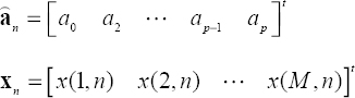
Let us consider that X₁(n), x₂(n)...x_N(n) represent M ECG beats of an ECG signal. Each i^th beat is expressed by a vector x_i.

The first beat is considered as a reference. It is denoted x_m:

Thus, each beat x_i i=2, ...M is considered obtained from the convolution between an impulsional signal z_i and the reference signal x_m.

This can be expressed as follows:

where X_m is a matrix having a Toeplitz structure, obtained from x_m and b_i is a zero-mean Gaussian noise vector.

The problem then consists of identifying z_i. In fact, the more significant the correlation is between x_i and x_m, the more z_i converges to an impulsional signal. The idea of the compression then consists of concentrating the information of a given ECG beat in a pseudo-impulse.

From equation [6.8], z_i can be estimated using the least squares by minimizing the Euclidian distance. In this case, the solution is given by:

Figure 6.4. Using the first ECG beat as an impulse response of the cardiac system, each recorded beat is deconvolved using the reference beat in order to estimate the pseudo-impulse (this is a typical inverse problem which necessitates regularization)

Figure 6.5 represents an original ECG signal. Using the first beat as a reference, the deconvolution of this signal, represented in Figure 6.6, clearly shows the impulsional aspect. In the next step, a simple thresholding of the low amplitudes is achieved as shown in Figure 6.7. This allows us to increase the number of zero values. For transmission purposes, only the non-zero samples are coded.

On reception, the ECG signal is reconstructed using a simple convolution with the reference beat (see Figure 6.8). It is obvious that for such a transmission mode, the reference signal should be transmitted before transmitting the impulsional signal.

Figure 6.5. Original ECG signal

Figure 6.6. Signal obtained after deconvolution using the first beat

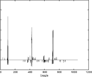
Figure 6.7. Thresholding of the deconvolved signal

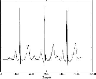
Figure 6.8. Reconstruction of the ECG signal using the thresholded impulsional signal

6.4.4.2. Compression of the ECG in the frequency domain

As presented in section 6.4.4.1, the proposed approaches are based on the parametrical modeling of the ECG signal in the time domain. In this section, the idea consists of modeling the transform of the ECG signal such as the DCT or the Fourier transform.

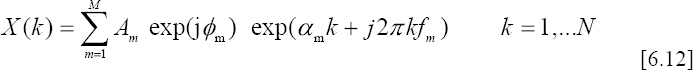
In Figures 6.9 and 6.10, we represent respectively the DCT of a normal ECG beat and the DCT of the PVC. We can observe that the obtained curves have a damped sinusoid aspect. Thus, the idea consists of modeling them mathematically as follows:

where:

– X(k) is the DCT of a segment of an ECG signal;

– M is the order of the model;

– N is the number of samples;

– are the amplitudes;

– α_m are the damping factors;

– f_m are the frequencies;

– φ_m [−π,π] are the initial phases;

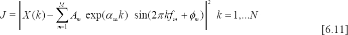
These parameters can be determined by minimizing the following criterion using any non-linear optimization technique. For instance, we can use a metaheuristic such as the genetic algorithms (GA).

After the convergence of the optimization algorithm, the estimated parameters are used to reconstruct the DCT model (Figure 6.11). Using the inverse Discrete Cosine Transform, we obtain the temporal ECG signal as shown in Figure 6.12.

Figure 6.9. DCT of a normal ECG beat

Figure 6.10. DCT of a PVC

Figure 6.11. [-] original DCT; [..] reconstructed DCT using 12 damped sinusoids

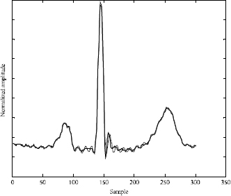
Figure 6.12. [-] original ECG beat; [..] reconstructed ECG beat

On the other hand, when calculating the Fourier transform of an ECG beat, we show that the curves corresponding to both the real part and the imaginary one, present as previously a damped sinusoid aspect. In this case, the problem is processed in the complex-domain without using any global optimization technique. In fact, some methods such as Prony are very appropriate for such situation.

The Discrete Fourier Transform of a given ECG signal is modeled as follows:

where as in the real case:

– M denotes the model order;

– N is the number of samples;

– are the amplitudes;

– α_m are the damping factors;

– are the frequencies;

– φ_m [−π,π] are the initial phases.

The problem consists of identifying the set of parameters .

The numerical results obtained from this approach applied to signals from the MIT-BIH database can be found in [OUA 06].

6.4.5. ECG compression for storage

As we have seen previously, the techniques presented so far are more appropriate to real time transmission than to storage. The compression ratio attained by these techniques varies from 15 to 20, depending of course on the required quality, the frequency sampling, the signal type (periodic, aperiodic, noisy, specific anomalies, etc.).

In this section, the presented approaches have been developed specifically for ECG storage. Thus, we will show how we can achieve very impressive compression ratios (i.e. 100 or more).

The first approach is presented in the section 6.4.5.1 and is based on the synchronization and the polynomial modeling of the dynamic of the ECG beats, whereas the second approach is based on the principle of the synchronization and interleaving (see section 6.4.5.2). Finally, an ECG compression technique that uses the standard JPEG 2000 will be presented in section 6.4.5.3.

When using these three techniques, the first step requires the separation of the ECG beats using any appropriate segmentation algorithm. Since the ECG signal is basically not periodic, the different segmented beats do not necessarily have the same duration. Therefore, in order to gather the set of ECG beats in a same matrix X so that each line contains one ECG beat, it is essential to perform an extrapolation of the different segments in order to equalize the durations. The variable N denotes here the size of the larger segment.

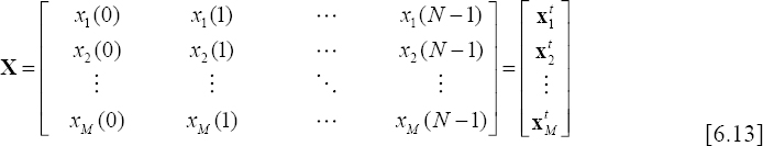
It is also important to be aware that the beats included in matrix X are highly correlated to each other. However, in order to minimize the fast transitions (i.e. high frequencies), the beats should be aligned (i.e. synchronized). In other words, we have to reduce the high frequencies which can occur between successive beats as shown respectively in Figures 6.13 and 6.14 representing one column of matrix X).

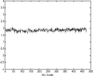
Figure 6.13. Low frequencies after synchronizing the ECG beats

Figure 6.14. High frequencies for non-synchronized ECG beats

Synchronization can be obtained easily using some basic correlation techniques.

6.4.5.1. Synchronization and polynomial modeling

The transform which leads to matrix X allows us to represent the ECG signal as an image. The non-stationarity of the ECG generally due to arrhythmias leads to a desynchronized surface as depicted in Figure 6.15. Since for an abnormal ECG signal, the shape of some beats might be time-variant, it is then essential to include a pre-processing phase which consists of gathering similar shapes in the same matrix. For example, suppose an ECG signal contains both normal beats and PVCs. In such a situation, the original matrix should be decomposed into two matrices so that each matrix contains only one specific beat type. The beats in each matrix should be synchronized; see Figure 6.16 for normal beats and Figure 6.17 for PVCs.

Now, since each row of the obtained matrixes contain a single beat, the processing technique consists of projecting each column on a polynomial basis as follows:

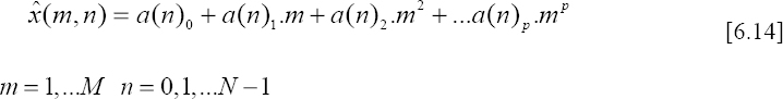
where a(n)_i represents the i^th coefficient of the p order polynomial at instant n.

Figure 6.15. Image representation of the ECG signal. Each row contains one ECG beat. Since the signal is not periodic, the obtained surface is desynchronized

These coefficients can be easily estimated using a least squares criterion:

Using a vectorial representation, the coefficients of each polynomial corresponding to the n^th column are estimated by:

where:

The final solution is given by:

where C is the classical Vandermonde matrix, expressed as follows:

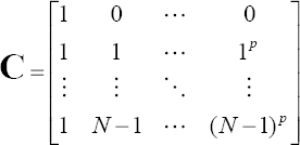
The polynomial _n is calculated using the following equation:

By projecting matrix X on the same polynomial basis, another matrix of coefficients, denoted A is derived. This is given by:

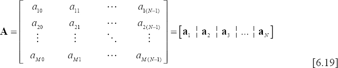
From this equation, we can note that the size of the matrix is A p × N whereas it is M × N for matrix X. Therefore, we can only store matrix A with the possibility of estimating the elements of matrix X allowing of course the reconstruction of the ECG signal.

The compression ratio obtained by this technique depends of course on the polynomial order as well as the number of samples of the longest segment.

As mentioned previously, when the ECG beats are synchronized, the variance in each column is considerably small. This also leads to a reduced polynomial order. In Figure 6.18, we show one column of a matrix composed of 480 ECG beats, projected on a six order polynomial basis. In fact, these six coefficients can reproduce up to “infinity” the tendency of whatever the number of ECG beats. Consequently, high compression ratios can be achieved with this technique. On the other hand, when the shape of the beats change, the approach becomes less interesting as shown in Figure 6.19. In fact, the reduced polynomial order cannot reproduce some abrupt changes. Therefore, a classification (as mentioned previously) of beats becomes in this case the most appropriate solution in order to overcome this disadvantage.

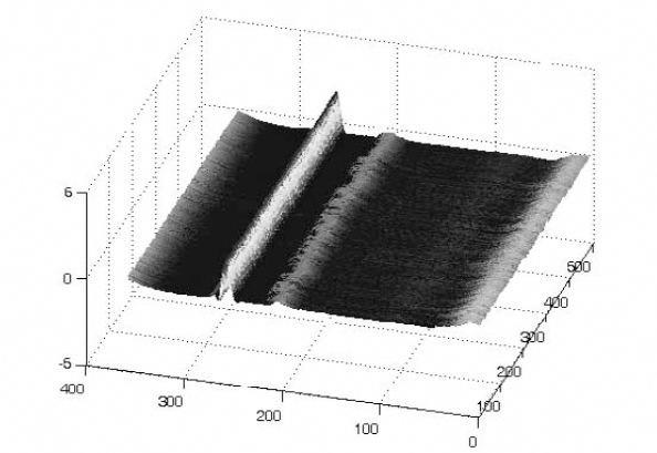
Figure 6.16. The alignment of the ECG beats reduces the high frequencies

Figure 6.17. Alignment of PVCs

Figure 6.18. Polynomial modeling of the low frequencies after ECG beat synchronization

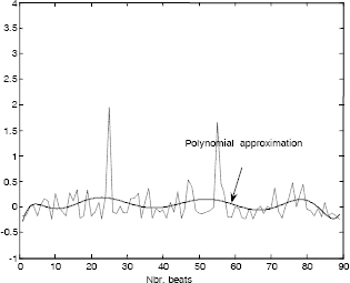
Figure 6.19. Polynomial modeling with a reduced order (non-synchronized case)

6.4.5.2. Synchronization and interleaving

This technique is simple in the sense that it uses matrix X [6.13] after synchronizing the ECG beats (in each row). However, an interleaving of these rows is then achieved in order to obtain a single signal denoted z, having the following structure:

Since the ECG beats have correlated shapes, the resulting signal z has a M × N size. Therefore, the shape of the obtained signal becomes very close to that of a single beat (Figure 6.20). Signal z seems to be noisy due to the variations between each beat. At this stage of processing, no compression is performed since it is only a transformation matrix-vector.

Figure 6.20. Signal obtained after ECG beat interleaving

A decomposition of signal z on a wavelet basis using three levels, allows an interesting separation of low frequencies (approximations cA₃) and high frequencies (details cD₃, cD₂, cD₁). Signal z_w is then obtained by:

Signal cA₃ can easily be characterized using a parametrical Gaussian model (section 6.4.4.1.1). Moreover, the low amplitudes related to the details cD₃, cD₂, cD₁ should be thresholded in order to create zero value blocks which can easily be coded. The numerical results obtained by applying those approaches on real signals are presented in [NAI 06].

6.4.5.3. Compression of the ECG signal using the JPEG 2000 standard

The most recent techniques for compressing the ECG signal consist of transforming the signal to an image before the coding operation. However, the standard JPEG 2000, initially dedicated to compressing images, has been successfully used to compress ECG signals. As in the previous technique, a preprocessing technique is required which consists of synchronizing the beats initially stored in a matrix X. Decoding the data requires of course the use of the parameters (delays) used for synchronization purposes; for more details about this technique, see [BIL 03].

6.5. Conclusion

Throughout the course of this chapter, several recent compression techniques basically dedicated to the ECG signal have been presented. The choice of method of course depends on the condition of recording.

Based on the results published, the compression ratio changes from 15 to 20. These rates can be significantly exceeded when the compression is performed for storage rather than for real-time transmission. In fact, this seems to be logical because when storage is required, past and future correlations can be taken into account.

Finally, it seems important to point out that the standardization of the techniques of compression dedicated to physiological signals seems to be delayed in relation to the progress achieved for the image. This might be a challenge for the future.

6.6. Bibliography

[AGA 01] AGARVAL R., GOTMAN J., “Long-term EEG compression for intensive-care setting”, IEEE Eng. in Med. and Biol., vol. 9, p. 23-29, 2001.

[AHM 01] AHMEDA S., ABO-ZAHHAD M., “A new hybrid algorithm for ECG signal compression based on the wavelet transformation of the linearly predicted error”, Med. Eng. Phys., vol. 23, p. 117-26, 2001.

[ALS 01] ALSHAMALI A., AL-SMADI A., “Combined coding and wavelet transform for ECG compression”, J. Med. Eng. Technol., vol. 25, p. 212-216, 2001.

[ALS 03] ALSHAMALI A., ALFAHOUM A., “Comments on an efficient coding algorithm for the compression of ECG signals using the wavelet transform”, IEEE Trans. Biomed. Eng., vol. 50, p. 1034-1037, 2003.

[ANT 97] ANTONIOL G., TONNELA P., “EEG data compression techniques”, IEEE Eng. in Med. and Biol., vol. 44, 1997.

[ASM 94] ASTM E1467-94, American Society for Testing and Materials, STM, (www.astm.org), 1916 Race St., Philadelphia, PA 19103, USA, 1994.

[BAT 01] BATISTA L., MELCHER E., CARVALHO L., “Compression of ECG signals by optimized quantization of discrete cosine transform coefficients”, Med. Eng. Phys., vol. 23, p. 127-34, 2001.

[BIL 03] BILGIN A., MARCELLIN M., ALTBACH M., “Compression of ECG Signals using JPEG2000”, IEEE Trans. on Cons. Electr., vol. 49, p. 833-840, 2003.

[BOR 05] BORSALI R., NAIT-ALI A., “ECG compression using an ensemble polynomial modeling: comparison with the wavelet based technique”, Biomed. Eng., Springer-Verlag, vol. 39, no. 3, p. 138-142, 2005.

[CAR 04] CARDENAS-BARRERA J., LORENZO-GINORI J., RODRIGUEZ-VALDIVIA E., “A wavelet-packets based algorithm for EEG signal compression”, Med. Inform. Intern. Med., vol. 29, p. 15-27, 2004.

[CEN 95] File Exchange Format for Vital Signs, Interim Report, Revision 2, TC251 Secretariat, Stockholm, Sweden, CEN/TC251/PT-40, 2000.

[CHA 05] CHATTERJEE A., NAIT-ALI A., SIARRY P., “An Input-Delay Neural Network Based Approach For Piecewise ECG signal compression”, IEEE Trans. Biom. Eng., vol. 52, p. 945-947, 2005.

[CHE 04] CHEN W., HSIEH L., YUAN S., “High performance data compression method with pattern matching for biomedical ECG and arterial pulse waveforms”, Comp. Method. Prog. Biomed., vol. 74, 2004.

[CLA 02] CLAVIER L., BOUCHER J.-M., LEPAGE R., BLANC J.-J., CORNILY J.-C., “Automatic P-wave analysis of patients prone to atrial fibrillation”, Med. Biol. Eng. Comput., vol. 40, p. 63-71, 2002.

[ENV 96] ENV 1064 Standard communications protocol for computer-assisted electrocardiography, European Committee for Standardisation (CEN), Brussels, Belgium, 1996.

[GAC 03] GACEK A., PEDRYCZ W., “A genetic segmentation of ECG signals”, IEEE Trans. Biomed. Eng, vol. 50, p. 1203-1208, 2003.

[GIU 02] GIURCANEANU C., TABUS I., MEREUTA S., “Using contexts and R-R interval estimation in lossless ECG compression”, Comput. Meth. Prog. Biomed., vol. 67, p. 17786, 2002.

[HAN 01] HANG X., GREENBERG N., QIN J., THOMAS J., “Compression of echocardiographic scan line data using wavelet packet transform”, Comput. Cardiol., vol. 28, p. 425-7, 2001.

[KEM 92] KEMP B., VÄRRI A., ROSA A.-C., NIELSEN K.-D., GADE J., “A simple format for exchange of digitized polygraphic recordings”, Electroencephalogr. Clin. Neurophysiol., vol. 82, p. 391-393, 1992.

[KOS 04] KOSKI A., TOSSAVAINEN T., JUHOLA M., “On lossy transform compression of ECG signals with reference to deformation of their parameter values”, J. Med. Eng. Technol., vol. 28, p. 61-66, 2004.

[LU 04] LU M., ZHOU W., “An EEG compression algorithm based on embedded zerotree wavelet (EZW)”, Space Med. Eng., vol. 17, p. 232-234, 2004.

[MIA 01] MIAOU S. YEN H., “Multichannel ECG compression using multichannel adaptive vector quantization”, IEEE Trans Biomed. Eng., vol. 48, p. 1203-1209, 2001.

[MIA 02] MIAOU S., LIN C., “A quality-on-demand algorithm for wavelet-based compression of electrocardiogram signals”, IEEE Trans Biomed. Eng., vol. 49, p. 233-9, 2002.

[MIA 05] MIAOU S., CHAO S., “Wavelet-based lossy-to-lossless ECG compression in a unified vector quantization framework”, IEEE Trans Biomed. Eng., vol. 52, p. 539-543, 2005.

[NAI 07a] NAÏT-ALI A., BORSALI R., KHALED W., LEMOINE J., “Time division multiplexing based-method for compressing ECG signals: application for normal and abnormal cases”, Journal of Med. Eng. and Tech., Taylor & Francis, vol. 31, no. 5, p. 324-331, 2007.

[NAI 07b] NAÏT-ALI A., “A New Technique for Progressive ECG Transmission using Discrete Radon Transform”, Int. Jour. Biomedical Sciences, vol. 2, pp. 27-32, 2007.

[NUN 05] NUNES J.-C., NAIT-ALI A., “ECG compression by modeling the instantaneous module/phase of its DCT”, Journal of Clinical Monitoring and Computing, Springer, vol. 19, no. 3, p. 207-214, 2005.

[NYG 01] NYGAARD R., MELNIKOV G., KATSAGGELOS A., “A rate distortion optimal ECG coding algorithm”, IEEE Trans Biomed. Eng, vol. 48, p. 28-40, 2001.

[OUA 07] OUAMRI A., NAIT-ALI A., “ECG compression method using Lorentzian functions Model”, Digital Signal Processing, vol. 17, p. 319-326, 2007.

[RAJ 02] RAJOUB B., “An efficient coding algorithm for the compression of ECG signals using the wavelet transform”, IEEE Trans Biomed. Eng., vol. 49, p. 355-362, 2002.

[ROD 04] RODRIGUEZ M., AYALA A., RODRIGUEZ S., DIAZ-GONZALEZ M., “Application of the Max-Lloyd quantizer for ECG compression in diving mammals”, Comp. Meth. Prog. Biomed, vol. 73, p. 13-21, 2004.

[WEI 01] WEI J., CHANG C., CHOU N., JAN G., “ECG data compression using truncated singular value decomposition”, IEEE Trans Inf. Tech. Biomed., vol. 5, p. 290-299, 2001.