
10
Modular Analysis: Computing with Curves
In the previous part, the concepts to compute the performance bounds in one server have been introduced. The aim of this part is to use them to study more complex communication networks. The general problem of computing performance bounds in networks has received much attention, and many techniques have been used, depending on the hypothesis on the arrival and departure processes.
This part is divided into three chapters. The first two chapters focus on the general methods to compute performance bounds in feed-forward networks (i.e. there is no cyclic dependence between the flows circulating in the network). Feed-forward networks are a general class of networks for which the stability condition (i.e. the condition under which the amount of data in the network remains bounded) is known. As a result, the only problem that is focused on here is the problem of computing performance bounds that approach as much as possible the exact worst-case performance bound. The third chapter will be devoted to cyclic networks, where no general result is known for the stability of large classes of networks.
As far as acyclic networks are concerned, there are two main approaches:
- 1) the first uses the contracts (arrival and service curves) to compute worst-case delay bounds. As we will see, the tightness of the performance bounds we had in the single server case is lost, but the methods developed are very algorithmically efficient. The key tool is the algebraic translation of the serialization of servers as a (min,plus) convolution. This is the object of this chapter;
- 2) the second directly uses the trajectories of flow satisfying the contracts. As a result, the results are far more precise. This has two consequences: in some cases, it is possible to obtain the exact worst-case performance bounds. This will be the aim of Chapter 11.
In this chapter, we focus on the performance bounds in networks that can be computed using the (min,plus) framework defined in the previous chapters. We focus on the computation of worst-case delays for a given flow or the worst-case backlog at a server and on acyclic networks.
Several methods can be used, but they rely on the same elements (for the delay computation here):
- 1) sort the servers in a topological order so that they are analyzed in this order;
- 2) for each server, compute the residual service curves for each flow and compute the intermediate arrival curves for each flow at the exit of this server;
- 3) compute a global service curve and an upper bound of the end-to-end delay for each flow.
Step 1 can be easily performed in linear time in the size of the network, by a depth-first-search algorithm, for example (see [COR 09]). Step 2 is carried out using the results of Chapters 5 and 7, and the computation depends on the service policy. Moreover, if a maximum service curve is known, then this step can be improved using grouping techniques. Step 3 is carried out using the algebraic properties of the convolution. In this chapter, Step 3 and improvements for Step 2 are detailed.
The chapter is organized as follows: we first present the network model and notations that we will use in this part of the book. Section 10.3 is devoted to the special case of nested tandems, for which better bounds can be obtained using the pay multiplexing only once phenomenon. Then, several general algorithms for computing performance bounds in feed-forward networks will be presented in section 10.4, from the naive to the elaborated ones. Finally, in section 10.5, we will prove the NP-hardness of computing exact worst-case delay bounds given the characteristics of the network.
10.1. Network model
10.1.1. Network description and notations
In our model, a network ![]() of n servers and m flows is described by several elements.
of n servers and m flows is described by several elements.
Flows. For all i in {1,…, m}, flow i is described by an arrival curve αi and a path ![]() where
where ![]() .
.
We write h ∈ pi or i ∈ Fl(h) if there exists ![]() such that
such that ![]() . With a slight abuse of notation, we also interpret pi as the set of servers crossed by the flow. If h = pi(ℓ), then predi(h) = pi(ℓ — 1), with the convention that if ℓ = 1, then predi(h) = 0.
. With a slight abuse of notation, we also interpret pi as the set of servers crossed by the flow. If h = pi(ℓ), then predi(h) = pi(ℓ — 1), with the convention that if ℓ = 1, then predi(h) = 0.
We also note fst(i) = pi(1) the first server visited by i, and end(i) the last system visited by i, i.e. pi(ℓi). Bits of data of flow i successively cross each server of pi in the order given by the path.
The cumulative arrival process of flow i before its visited server is denoted by ![]() and is αi-constrained. For h ∈ Pi, we denote by
and is αi-constrained. For h ∈ Pi, we denote by ![]() the cumulative departure process of flow i after server h.
the cumulative departure process of flow i after server h.
Servers. For all h in {1,…,n}, server ![]() – or simply server h – is described by a service curve β(h) ∈
– or simply server h – is described by a service curve β(h) ∈ ![]() , a type of service
, a type of service ![]() (strict or min-plus) and a service policy (this can be arbitrary, FIFO, static priorities, general processor sharing, for example). For each server h ∈ {1,…,n}, the aggregate server is
(strict or min-plus) and a service policy (this can be arbitrary, FIFO, static priorities, general processor sharing, for example). For each server h ∈ {1,…,n}, the aggregate server is ![]() .
.
With the notations introduced above, we have that for all h ∈ {1,…, n},
For server h and ![]() , we denote by Starth (t) the start of the backlogged period of server h at time t.
, we denote by Starth (t) the start of the backlogged period of server h at time t.
The graph induced by this network is the directed graph ![]() = (V, E), where V = {1,…,n} is the set of the servers and E =
= (V, E), where V = {1,…,n} is the set of the servers and E = ![]() , pi =
, pi = ![]() is the pair of consecutive servers on a flow. As a result,
is the pair of consecutive servers on a flow. As a result, ![]() is a directed and simple graph (with no loop and no multiple edge).
is a directed and simple graph (with no loop and no multiple edge).
10.2. Some special topologies
In this part, we will focus on some topologies illustrated in Figure 10.1.
Feed-forward networks. A feed-forward network is a network ![]() whose induced graph
whose induced graph ![]() is acyclic. In that case, it is possible to number the servers so that the path of each flow is increasing: ∀i ∈ { 1,…, m},
is acyclic. In that case, it is possible to number the servers so that the path of each flow is increasing: ∀i ∈ { 1,…, m}, ![]() . This numbering can be obtained by performing a topological sort (see, for example, [COR 09]). We will always assume this type of numbering when dealing with acyclic networks (in Chapters 10 and 11).
. This numbering can be obtained by performing a topological sort (see, for example, [COR 09]). We will always assume this type of numbering when dealing with acyclic networks (in Chapters 10 and 11).
Tandem networks. A tandem network is a special case of feed-forward network with a line topology: the edges of the induced network are (h, h + 1), h ∈ {1,…, n − 1}. As a result, the path of each flow is of the form 〈fst(i), fst(i) +1,…, end(i)〉.

Figure 10.1. Examples of topologies of networks. Top: a feed-forward network but not tandem; middle: a tandem network but not nested; bottom a nested tandem network. For a color version of this figure, see www.iste.co.uk/bouillard/calculus.zip
Nested tandem networks. Finally, a nested tandem network is a tandem network such that the path of each flow is included in the path of the other. Then, the flows can be numbered so that
10.3. The pay multiplexing only once phenomenon
Consider the network of Figure 10.2, with two flows crossing two servers.

Figure 10.2. Network with two flows and two servers to illustrate the pay multiplexing only once phenomenon. For a color version of this figure, see www.iste.co.uk/bouillard/calculus.zip
Suppose that in the first server, a burst of data of flow 1 is served before the data of flow 2, although data of flow 2 arrived before the burst in the server. Then, in the second server, this burst of data of flow 1 cannot overtake the data of flow 2 again, as it already arrived before in the second server. However, when we apply Theorems 6.1 and 7.1, we obtain the residual min-plus service curve
where ![]() is the arrival curve flow 1 at server 2. In this formula, the multiplexing of the two flows appears in the two servers, meaning that a bit of data can suffer from the same burst of flow 1 in each server, which is too pessimistic. In some cases, however, direct computation gives better results.
is the arrival curve flow 1 at server 2. In this formula, the multiplexing of the two flows appears in the two servers, meaning that a bit of data can suffer from the same burst of flow 1 in each server, which is too pessimistic. In some cases, however, direct computation gives better results.
Indeed, suppose that the service curves are strict and that the service policy is blind. Let t ∈ ![]() . We can define s = Start2 (t) and u = Start1 (s), the respective start of backlog period of t at server 2 and of s at server 1. We can write:
. We can define s = Start2 (t) and u = Start1 (s), the respective start of backlog period of t at server 2 and of s at server 1. We can write:

inducing

and ![]() = (β(1) * β(2) − α1)+ is a service curve for flow 2. We call this the pay multiplexing only once (PMOO) phenomenon.
= (β(1) * β(2) − α1)+ is a service curve for flow 2. We call this the pay multiplexing only once (PMOO) phenomenon.
This concept was introduced by Schmitt et al. in [SCH 08a, SCH 08b, SCH 06b, SCH 07], and it can be noted that this result cannot be found by applying Theorem 6.1 and then Theorem 7.1 as the service curve obtained by Theorem 6.1 is not strict. However, this example shows that direct computation gives the same result.
10.3.1. Loss of tightness
The PMOO phenomenon could be generalized to an arbitrary network, but this is not the solution to always compute better performance bounds, although this intuitively should be the case as the burst of flow 1 is counted only once. In this section, we illustrate the difficulty of getting good bounds.
We still consider the small network of Figure 10.2 with the following parameters:
- – for h ∈ {1, 2}, server h offers a strict service curve
 , and for each server, the service is arbitrary;
 - – for i ∈ {1,2}, flow i is constrained by the arrival curve
 , and compare the two service curves obtained,
  and
and  .
.

and
If β1 = β2, then ![]() . But if b1 = 0, T1 = 0 and R2 > R1, then
. But if b1 = 0, T1 = 0 and R2 > R1, then ![]() .
.
The first method, used to compute ![]() , can be generalized for general feed-forward networks. This is the object of section 10.4. The second method, leading to
, can be generalized for general feed-forward networks. This is the object of section 10.4. The second method, leading to ![]() , cannot be generalized in such a simple way when more flows interfere, and especially when the flows are not nested. The following section shows that the formula can be generalized for tandem networks under arbitrary multiplexing. This result might be difficult to apply to specific service policies. One reason, illustrated in section 10.3.3, is that service policies are not stable under composition of servers. However, in section 10.3.4, we show how to benefit from the PMOO phenomenon in nested tandem for static priority and FIFO policies. Another way to generalize this approach is to use linear programming. Indeed, it follows more or less the same computing scheme: first work with the trajectories and bound, using the arrival and service curves only in the last step. This will be discussed in Chapter 11.
, cannot be generalized in such a simple way when more flows interfere, and especially when the flows are not nested. The following section shows that the formula can be generalized for tandem networks under arbitrary multiplexing. This result might be difficult to apply to specific service policies. One reason, illustrated in section 10.3.3, is that service policies are not stable under composition of servers. However, in section 10.3.4, we show how to benefit from the PMOO phenomenon in nested tandem for static priority and FIFO policies. Another way to generalize this approach is to use linear programming. Indeed, it follows more or less the same computing scheme: first work with the trajectories and bound, using the arrival and service curves only in the last step. This will be discussed in Chapter 11.
10.3.2. A multi-dimensional operator for PMOO
In this section, we generalize the PMOO principle to any tandem network. This result is taken from [BOU 08a].
THEOREM 10.1 (PMOO multi-dimensional operator).– Consider a tandem network ![]() where flow 1 crosses all of the servers. If each server h offers a strict service curve β(h), with the same assumptions and notation as above, a min-plus service curve offered for flow 1 is:
where flow 1 crosses all of the servers. If each server h offers a strict service curve β(h), with the same assumptions and notation as above, a min-plus service curve offered for flow 1 is:

We first prove a lemma that concerns the cumulative processes.
LEMMA 10.1.– With the previous assumptions and notation, ![]() such that
such that

Moreover, ![]() .
.
PROOF.– To ease the notations, we will identify ![]() with
with ![]() .
.
Set sn+1 = t and for all h ∈ {1,…,n}, define sh = Starth(sh+1) and uh = sh+ 1 — sh.
Since the servers offer strict service curves, we have that for all servers h,
Summing all those inequalities and collecting terms with regard to flow indices, we get

By removing the terms present on both sides, it simplifies into:

which gives the first inequality of the lemma, since ![]() .
.
Moreover, we have for all flow i, ![]() , so
, so ![]() , which gives the second inequality.
, which gives the second inequality.
□
We can deduce from this lemma a residual service curve provided to flow 1 for its whole path.
PROOF OF THEOREM 10.1.– Consider the inequalities proved in Lemma 10.1. We clearly have ∀i ∈ {1….,m}, ∀h ∈ {fst(i),…,end(i)}, ![]() . Moreover, for all 2
. Moreover, for all 2 ![]() ,
,

Thus,

From Lemma 10.1, we also have ![]() . As a result of those two inequalities, we have
. As a result of those two inequalities, we have ![]() , where β is the function defined above.
, where β is the function defined above.
□
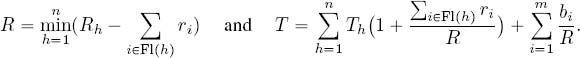
EXAMPLE 10.1.– To illustrate the PMOO phenomenon, consider the network of Figure 10.1 (middle), which is the example detailed by Schmitt et al. in [SCH 06b, section 4]. Theorem 10.1 provides the following service curve for the path:

This result introduces a multi-dimensional operator for network calculus. It generalizes Theorem 7.1, which tackles paths with a single node and a unique cross-traffic flow. When service curves are rate-latency (![]() ) and the arrival curves are leaky-buckets
) and the arrival curves are leaky-buckets ![]() , the formula becomes:
, the formula becomes:


with ![]() , which is a convex function composed of two segments: a segment of slope – ∑i∈FI(h)
, which is a convex function composed of two segments: a segment of slope – ∑i∈FI(h) ![]() between 0 and Tj and an infinite segment of slope Rh ‒ ∑i∈FI(h)
between 0 and Tj and an infinite segment of slope Rh ‒ ∑i∈FI(h) ![]() . Therefore,
. Therefore, ![]() can be easily computed using Theorem 4.1. The finite segments have negative slopes, and we are interested only in the part where the convolution is greater than
can be easily computed using Theorem 4.1. The finite segments have negative slopes, and we are interested only in the part where the convolution is greater than ![]() bi, which is of slope
bi, which is of slope ![]() . After computation, we obtain that β = βR,T, with
. After computation, we obtain that β = βR,T, with
10.3.3. Composition and service policies
WARNING.– The PMOO phenomenon must be used with care. Indeed, the previous theorem does not imply that a system composed of two servers with the same service policy obeys this service policy. It is true in a few special cases: blind multiplexing (this is obvious as there is no assumption for the service policy) and FIFO multiplexing. Indeed, if a bit of data a arrives before a bit of data b, then a will depart from the first server before b, and the same will hold for server 2.
However, this is not true for other service policies. Let us illustrate this fact with two service policies: static priority (SP) and generalized processor sharing (GPS). In the following example, we consider the simple network in Figure 10.2.
- ‒ Static priority: this can be deduced from the fact that the end-to-end service curve of two servers in tandem is not a strict service curve. Consider Figure 6.5 and suppose that the flow drawn is the one that is given the highest priority. Consider now a second flow (with lower priority). As the service curves are pure delays, if data from the second flow arrive at time 0, those data will exit at time T1 + T2. But at that time, flow 1 is still backlogged, which means that the system composed of the two servers is globally not a static priority server.
- ‒ Generalized processor sharing: take
 and
and  the proportion of service guaranteed for flows 1 and 2 for each server. Suppose that the first flow arrives according to α1 and that half of the burst is served at once, at time 0+. Flow 2 arrives from time 1, according to α2(t − 1). Between times 0 and 1, only flow 1 is served. From time 0+, the servers serve data exactly according to their arrival curve. From time 1, server 1 is backlogged for both flows. Then, each flow arrives at rate 2 in server 2.
In server 2, flow 2 cannot be backlogged (it is guaranteed service rate 2.5), so is served at rate 2. Then, flow 1, which is backlogged, is served at rate 5 − 2 = 3. As a result, flow 2 is not guaranteed half of the service of the global system. One can invert the role of flows 1 and 2 and then can conclude that neither of the two flows can be guaranteed half of the service of the global system. Hence, the global system is not GPS.
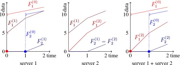
Figure 10.3. Two GPS servers in tandem is not a GPS server. For a color version of this figure, see www.iste.co.uk/bouillard/calculus.zip
10.3.4. Nested tandems
Nested tandem systems are a special case where PMOO can be generalized for several service policies. We already gave a general formula for blind multiplexing (Theorem 10.1), and in this section, we show that this phenomenon can be taken into account for fixed priorities and FIFO service policies. Intuitively, this is possible when flows can be removed one by one, from the nested to the longest. Two cases are explored: the nested flows are given a higher priority (equation [10.1] can be directly applied) or the service policy is FIFO, because the service policy is preserved by the composition of servers.
10.3.4.1. Static priorities and PMOO
Suppose that a nested tandem respecting the numbering (Nest) is crossed by m flows and that static priority is at work, respecting the priority rule that flows with the highest number have the lowest priority. In other words, if pi ⊆ pj, then flow i has higher priority than flow j. The service curves ![]() for each flow i can be computed using Algorithm 3. This is a straightforward generalization of equation [10.1], and the proof is similar to that of Theorem 10.1, so we do not give details here. A more rigorous proof can be found in [BOU 09].
for each flow i can be computed using Algorithm 3. This is a straightforward generalization of equation [10.1], and the proof is similar to that of Theorem 10.1, so we do not give details here. A more rigorous proof can be found in [BOU 09].
EXAMPLE 10.2.– Consider the nested network at the bottom of Figure 10.1. We compute
10.3.4.2. FIFO and PMOO
The same can be done for FIFO multiplexing using the residual service curves thanks to the following three facts:
- 1) only min-plus service curves are considered;
- 2) the concatenation of FIFO servers in tandem results in an FIFO system;
- 3) when considering only a subset of flows, the service policy among those flows only is also FIFO.
The following proposition is a direct consequence of Theorems 7.5 and 6.1, and is used recursively in Algorithm 4. The principle of this algorithm is the same as above: we remove the flows one by one, beginning with the most nested. For each flow, a new residual service curve is computed for the other flows. We use the following proposition.
PROPOSITION 10.1.– Consider a sequence of n FIFO servers offering respective min-plus service curves β(h) crossed by m flows. Suppose that flow 1 is constrained by the arrival curve α. Then, for all θ > 0,
is a min-plus service curve for the m ‒ 1 other flows.
A major drawback of this algorithm is that the parameters θi must be fixed in advance. If analytic formulas are obtained, then it is also possible to perform an optimization step by computing the values of (θi) which, for example, will give the least delay bound. This is in general a very difficult problem that has been extensively studied by Lenzini, Stea and others. In [LEN 06], it is proved that in the case of sink-tree tandem topologies (all flows stop at the last server), the optimal parameters can be computed recursively, and these parameters lead to a tight residual service curve, in the sense that a tight delay bound can be computed from the residual service curve. In [LEN 08], the approach is extended to any tandem topology by cutting flows in order to obtain a nested tandem. Finally, in [BIS 08], a simple example shows evidence that the tightness is obtained only for sink-tree topologies.

Figure 10.4. Sink-tree tandem network. For a color version of this figure, see www.iste.co.uk/bouillard/calculus.zip
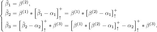
EXAMPLE10.3.– As an example of the optimization of parameters θ1, inspired by [LEN 06, Theorem 4.6], let us consider the very simple example of Figure 10.4, and let us compute the residual service curve that would be obtained for a flow crossing the two servers. We assume that arrival curve for flow i is ![]() constrained and that server h offers the min-plus service curve
constrained and that server h offers the min-plus service curve ![]() . We first compute
. We first compute
From Example 7.1, we can consider only values of θ1 that are greater than ![]() . The residual curve obtained is
. The residual curve obtained is
As a second step of the algorithm,![]() . First,
. First,![]() . Here again, we can discard values of θ2 that do not satisfy
. Here again, we can discard values of θ2 that do not satisfy ![]() , as they will not be optimal. Then, θ2 is lower bounded by
, as they will not be optimal. Then, θ2 is lower bounded by
Then, ![]() is of the form
is of the form ![]() with
with
Now, suppose that a flow constrained by the arrival curve![]() crosses this tandem network. The residual service curve for flow 3 is then
crosses this tandem network. The residual service curve for flow 3 is then ![]() . Under stability conditions (R1 > r2 + r3 and R2 > r1 + r2 + r3), the worst-case delay is found as
. Under stability conditions (R1 > r2 + r3 and R2 > r1 + r2 + r3), the worst-case delay is found as ![]() , i.e.
, i.e.
This delay depends on both θ1 and θ2, but we can first fix θ1 and compute the optimal value of θ2 for this fixed θ1, and finally optimize θ1.
After computations, we find that the optimal value for θ2 is ![]() . In that case,
. In that case, ![]() . Thus, it is easy to see that to minimize the maximal delay, θ1 has to be minimized, and θ1 = C1 = T2 +
. Thus, it is easy to see that to minimize the maximal delay, θ1 has to be minimized, and θ1 = C1 = T2 + ![]() . Finally, we find:
. Finally, we find:
10.4. Per-flow analysis of networks
In this section, we first give several ways to compute worst-case delay upper bounds, from the most naive method to more efficient ones.
10.4.1. Total output analysis
If only the results of Chapter 5 are used, a delay bound can be computed using Algorithm 5. It requests that the service curves are strict.
In line 3, α(h) is an arrival curve for the arrival cumulative function at server h. Once a flow is aggregated, there is no operation to compute curves for individual flows, hence the pessimism. Then, d(h) is the maximum delay suffered by a bit of data in a server offering a strict service curve β(h) and with arrival curve α(h). As the flow is an aggregation of several flows with no a priori service policy, this flow cannot be considered as FIFO, and the delay cannot be computed as the horizontal distance between the arrival and service curves. Instead, the maximum length of a backlogged period has to be considered, which corresponds to the formula of line 4 (Theorem 5.5).
This algorithm is very pessimistic as it does not take into account the service policies. Nevertheless, it can be used under very general assumptions: if FIFO-per-flow is not required, which is not possible for the other methods presented hereafter (note that when the flows are not FIFO, better methods exist; see, for example, [SCH 11]).
EXAMPLE 10.4.– Consider the non-tandem network in Figure 10.1 (top). We find

and the delays can be directly derived from these formulas.
Explained this way, the method is very pessimistic, especially because it computes performances as if all of the data served by a given server is transmitted to all of its successors. It is possible to circumvent this by using Theorem 5.4 and replacing line 3 with
or

depending on the shape of the arrival curves. A similar technique is used in [BON 16b].
It should be obvious that this method can be improved. This is done in several ways:
- 1) taking into account the FIFO-per-flow assumption and the service policy. For example, if the servers are FIFO, then line 4 can be replaced by d(h) = hDev(α(h), β(h)) and min-plus service curves can be considered;
- 2) taking into account the pay burst only once phenomenon, corresponding to the composition of servers, which is the object of the rest of the section;
- 3) taking into account the pay multiplexing only once phenomenon when possible, which was discussed in section 10.3.
10.4.2. Separated flow analysis
Algorithm 6 gives a generic way to compute performance bounds, taking into account the pay burst only once phenomenon. It first computes an arrival curve for each flow at each intermediate system: ![]() is an arrival curve for
is an arrival curve for ![]() . Then, it computes the residual service curve for each flow at each system:
. Then, it computes the residual service curve for each flow at each system: ![]() is the residual service curve for flow i at system h. Finally, it computes the global service curve for each flow by a convolution, and worst-case performance upper bounds can be computed using that curve and Theorem 5.2.
is the residual service curve for flow i at system h. Finally, it computes the global service curve for each flow by a convolution, and worst-case performance upper bounds can be computed using that curve and Theorem 5.2.
Algorithm 6 is valid for blind multiplexing (and thus for any other service policy) if the systems offer strict service curves. The performance bounds computed with this algorithm can be improved if more information is known about the systems and the curves.
- 1)If a maximum service curve
 and a shaper σ(h) is known for each server h, as well as a minimum arrival curve
  for each flow i, then lines (4–5) can be replaced by the following three lines (with obvious notations), following Theorem 5.3:

- 2) If the service policy is FIFO (server can offer a min-plus service curve), SP or GPS, it suffices to replace lines (4–5) with the formulas corresponding to the specific policy, i.e. using Theorems 7.5, 7.6 or 7.7. Naturally, it is possible to combine the different service policies with maximum service curves and minimum arrival curves.
The algorithm presented here does not claim optimality, but algorithmic efficiency. Indeed, it requires ![]() (nm) basic operations (convolution, deconvolution, etc.).
(nm) basic operations (convolution, deconvolution, etc.).
EXAMPLE 10.5.– Take the example of Figure 10.1 (top) again. We obtain:

If the service policy is static priority with flow 1 having the highest priority and flow 3 the lowest, then the computed arrival and service curves become:

10.4.3. Group flow analysis
Total output analysis and separated flow analysis consider either the whole set of flows crossing a server, or each flow individually. These are two extremal solutions, and grouping flows can be done in a more clever way. This is especially the case when a shaper σ(h) is known for each server h.
In TOA, when a flow is aggregated at a server, the whole worst-case backlogged bound is used for the next server. Moreover, it computes the worst-case delay for each server.
In SFA, a residual service curve per server and flow is obtained by using the formulas ![]() and
and ![]() , with
, with ![]() . This method can become very pessimistic when several flows follow the same arc in the network. Indeed, consider the network of Figure 10.1 (middle) and server 2. The arrival curves
. This method can become very pessimistic when several flows follow the same arc in the network. Indeed, consider the network of Figure 10.1 (middle) and server 2. The arrival curves ![]() and
and ![]() have been computed. When computing the service offered by server 2 to flow 3, we will compute
have been computed. When computing the service offered by server 2 to flow 3, we will compute ![]() . Another solution would be to compute the global arrival curve to server 2 from server 1, which is, from Theorem 5.3,
. Another solution would be to compute the global arrival curve to server 2 from server 1, which is, from Theorem 5.3, ![]() , and the residual service curve for flow 3 is thus
, and the residual service curve for flow 3 is thus ![]() .
.
The group flow analysis principle is to compute arrival curves for flows along the arcs of the network.
The same argument can be used for maximal service curves instead of shaping curves, but to keep things simple, only shaping curves will be discussed here. Similarly, this approach could be applied to any way of grouping flows. We restrict ourselves here to the grouping along the arcs of the network. It is a natural way of grouping, which takes advantage of the shaper. This way of grouping flows can potentially lead to an algorithm with an exponential complexity.

Figure 10.5. Grouping flows according to the arcs of the network: grouping flows f = {2, 3, 4} after server h requires them to be partitioned in two subsets f1 and f2 depending on their previous visited server. For a color version of this figure, see www.iste.co.uk/bouillard/calculus.zip
To generalize the above example, let us consider server h, depicted in Figure 10.5. To compute the residual service curve of flows in f and their arrival curve after server h, we need to know the arrival curve η of this group of flows and that of the other flows ![]() in order to use the formulas
in order to use the formulas
To compute the arrival curves η and ![]() , it is possible to group flows according to the arc they cross. For this, let us introduce an additional notation: Fl
, it is possible to group flows according to the arc they cross. For this, let us introduce an additional notation: Fl![]() is the set of flows that cross servers
is the set of flows that cross servers ![]() and k consecutively (equivalently, it is the set of flows that follow the arc
and k consecutively (equivalently, it is the set of flows that follow the arc ![]() ). Thus, we can now write the formula:
). Thus, we can now write the formula:
and similarly for ![]() by replacing f with
by replacing f with ![]() .
.

Figure 10.6. Network example for the group flow analysis. For a color version of this figure, see www.iste.co.uk/bouillard/calculus.zip
The group flow analysis is then performed in the following two steps, given by Algorithm 7:
- 1) Computing the group of flows that are needed for the analysis. This is done by a backward exploration on the servers. If the performance is computed for each flow i, we must compute the residual service curve for each flow i for each server crossed by it, hence the initialization line 2. Then, line 6 groups of flows to be evaluated at each server are computed following the example of Figure 10.5 for each server h.
- 2) Computing the residual service curves and arrival curves that are needed for the analysis of flow i. This is done server by server following the topological order. The first step ensures that all the needed grouping have been computed. Note that the empty set can be an element of Fh. We use the convention that
 .
.
Since the number of flow groups requested might be exponential, it might be useful to restrict to the computation of the residual service curve of a subset of flow of interest (e.g. a single flow i). In that case, only the initialization step line 2 is modified, by replacing ![]() with
with ![]() and ∅ otherwise.
and ∅ otherwise.
EXAMPLE10.6.– Take the example of Figure 10.6, where the flow of interest is flow 2. At the initialization step line 2, we get F2 = F3 = F4 = {{2}} and F1 = ∅. Then, backward computing of the groups gives (we do not take into account the empty sets that might appear): F4 = {{2}} (this is never modified), F3 = {{2}, {1,3}}, F2 = {{3}, {2,4}, {2}, {3,4}} and F1 = {{1}}.
Now we can compute the arrival curves and service curves:
In server 1, ![]() and
and ![]() .
.
In server 1, ![]() and
and ![]() , then.
, then.

In server 3,![]() and
and ![]() , then
, then

Finally, in server 4, we have ![]() and
and ![]() , then
, then
10.5. NP-hardness of computing tight bounds
In the previous sections, several ways of computing worst-case performance bounds have been described. The algorithms all have a polynomial complexity in the size of the network and in the number of basic operations performed (and these operations for the usual classes of functions have a polynomial complexity). However, it has also been shown in section 10.3.1 that it is not possible to obtain tight performance bounds. Here, tight means that it is possible to find cumulative departure and arrival processes that obey all of the constraints (arrival curves, service curves), such that the maximal delay of a flow or the maximum backlog is exactly the bound to be computed with the residual service curve obtained from the algorithm.
In this section, we show that the problem of finding the exact worst-case performance bound is an NP-hard problem, meaning that unless P = NP, there is no polynomial algorithm to solve the exact worst-case performance problem in the network calculus framework.
THEOREM 10.2. ‒ Consider a feed-forward network where every server has an arbitrary multiplexing service policy.
- ‒ computing the maximum backlog at a given server is NP-hard;
- ‒ computing the maximum delay of a flow is NP-hard.
PROOF.‒ We reduce the problem exact three-cover (X3C) to our problem. An instance of X3C is a collection ![]() of 3q elements and a collection
of 3q elements and a collection ![]() of s sets of three elements of
of s sets of three elements of ![]() . The problem is to decide whether there exists a cover of
. The problem is to decide whether there exists a cover of ![]() by q elements of
by q elements of ![]() . We will reduce this problem to deciding whether a given backlog or delay can be reached in a server of a network.
. We will reduce this problem to deciding whether a given backlog or delay can be reached in a server of a network.
From an instance of X3C, we build a network as shown in Figure 10.7. More precisely, the upper stage consists of 3q servers U1 ,…,U3q, all with strict service curve ![]() . The middle stage consists of s servers V1,…,Vs, all with strict service curve
. The middle stage consists of s servers V1,…,Vs, all with strict service curve ![]() . Finally, the lower stage has only one server V, with service curve
. Finally, the lower stage has only one server V, with service curve ![]() with R > 3s. There are 3s flows, each crossing three servers from top to bottom. Flow (i, j) crosses servers Vj, Vi and W if and only if uj ∈ vi. Each of those interfering flows has an arrival curve
with R > 3s. There are 3s flows, each crossing three servers from top to bottom. Flow (i, j) crosses servers Vj, Vi and W if and only if uj ∈ vi. Each of those interfering flows has an arrival curve ![]() (note that there can be no burst).
(note that there can be no burst).

Figure 10.7. Transformation of an instance of X3C into a network. For a color version of this figure, see www.iste.co.uk/bouillard/calculus.zip
The example of Figure 10.7 is with ![]() = {1,2, 3,4,5,6} and
= {1,2, 3,4,5,6} and ![]() = {{1,2, 3}, {2, 3,4}, {4,5,6}}, so {{1,2,3}, {4,5, 6}} is a 3-cover of
= {{1,2, 3}, {2, 3,4}, {4,5,6}}, so {{1,2,3}, {4,5, 6}} is a 3-cover of ![]() .
.
NP-hardness of the maximum backlog. We want to decide whether the backlog in W can be at least 3s — 2q.
We first prove that the worst-case backlog in server W will be obtained at time 1— when flows arrive according to α from time 0, and when servers Uj and Vi are exact servers on [0,1) and infinite at time 1. The backlog of server W at time 1 is then the backlog in the whole system at time 1—.
Fix 0 as the date of arrival of the first bit of data in the system.
The worst-case backlog is obtained at time s ![]() 1. If it were obtained at time s < 1, then every bit of data would not yet have been sent into the network, and if some backlog could be created at time s, some more can be created until time 1.
1. If it were obtained at time s < 1, then every bit of data would not yet have been sent into the network, and if some backlog could be created at time s, some more can be created until time 1.
The worst-case backlog is obtained at time s = 1. If it were obtained at time s > 1, consider the following transformation: delay the arrival of every flow so that every flow starts arriving at time s — 1. Then, the quantity of data served during [s — 1,s) after transformation is less than the quantity of data served during [0, s) in the initial configuration, hence the backlog has increased, and the first bit of data arrives at time s — 1 instead of 0 and there is a worst-case trajectory with s = 1.
Correspondence with X3C. Consider an infinitesimal time interval, during which each flow (i, j) at the upper stage is served at rate ![]() , with
, with ![]() . The service rate of Ui is
. The service rate of Ui is ![]() and then the growth rate of the backlog during that time interval at the middle stage is
and then the growth rate of the backlog during that time interval at the middle stage is ![]() . At the upper stage, a backlog is created at rate 3s —
. At the upper stage, a backlog is created at rate 3s — ![]() , which does not depend on the flows that are served. There is no backlog created at server V since R > 3s. Maximizing the backlog is equivalent to maximizing the following function:
, which does not depend on the flows that are served. There is no backlog created at server V since R > 3s. Maximizing the backlog is equivalent to maximizing the following function:
with the constraints: ∀ j ∈ {1,…, 3q}, ![]() and
and ![]() .
.
Our problem boils down to the maximization of a convex function on a convex set. The maximum values are then obtained at some extremal vertices of the convex set. The extremal vertices of the convex set are such that ![]() and then
and then ![]() . Maximizing our function is then equivalent to maximizing the number of i such that
. Maximizing our function is then equivalent to maximizing the number of i such that ![]() .
.
This number is upper-bounded by q, and this maximum is reached if and only if there is an X3C cover (in fact, there is a point-to-point correspondence between the set of extremal vertices that reach q and the set of X3C covers).
If there exists an X3C cover, then the backlog in the middle stage increases at rate q (at rate 1 for each server that receive data at rate 3). If there is no X3C cover, then the backlog in the middle stage increases at most at rate q — 1.
Finally, the above reasoning is valid for the interval of time [0,1). Indeed, the backlog is sub-additive: if an arrival cumulative function F1 defined on the interval [0, s] in a server creates a backlog b1 at time s, and if the arrival cumulative function F2 such that F2(s) = 0 creates a backlog b2 at time t ![]() s (when the server is empty at time s), then the process F1 + F2 creates a backlog b
s (when the server is empty at time s), then the process F1 + F2 creates a backlog b ![]() b1 + b2 at time t. As a result, there is no advantage to changing the service rates
b1 + b2 at time t. As a result, there is no advantage to changing the service rates ![]() during the interval of time [0,1). At time 1, servers Uj and Vi serve all of their backlog and the backlog in server W is then at most 3s − 2q. This maximum is reached if and only if there is an X3C cover. If there is no X3C cover, then the backlog is at most 3s − 2q − 1.
during the interval of time [0,1). At time 1, servers Uj and Vi serve all of their backlog and the backlog in server W is then at most 3s − 2q. This maximum is reached if and only if there is an X3C cover. If there is no X3C cover, then the backlog is at most 3s − 2q − 1.
NP-hardness of the delay. We keep the same scheme of reduction. There is an additional flow crossing server W only and we are now interested in computing the worst-case delay for a bit of data of that flow (we can take ![]() with
with ![]() < R − 3s and the maximum delay can be obtained for the first bit of data arriving in the system).
< R − 3s and the maximum delay can be obtained for the first bit of data arriving in the system).
The worst-case scenario for that network first creates a backlog in server W and then considers every other server as an infinite capacity server. To create the backlog, we use the previous construction.
Backlog at a server of the upper stage can be created if data arrive at a rate more than 1.
Backlog at a server of the middle stage can be created if there is an arrival rate of ![]() > 2 at a server of the middle stage. The backlog grows at rate
> 2 at a server of the middle stage. The backlog grows at rate ![]() − 2. If the arrival rate is exactly 3, then the flows arrive at rate 1, blocking the flows at the upper level, and so this is the scenario that builds the greatest backlog.
− 2. If the arrival rate is exactly 3, then the flows arrive at rate 1, blocking the flows at the upper level, and so this is the scenario that builds the greatest backlog.
Suppose that exactly k servers of the middle stage have an arrival rate of 3 between time 0 and tk. Without loss of generality, the servers that create backlog are V1,…,Vk. The backlog created is (Nk − 2k)tk, where ![]() and for the other flows, either they are idle or data are transmitted. For these other flows, no backlog is created at the middle stage, but some backlog can be built at the upper stage at rate
and for the other flows, either they are idle or data are transmitted. For these other flows, no backlog is created at the middle stage, but some backlog can be built at the upper stage at rate ![]() for each server Cj. We can upper-bound the backlog created by using the inequality
for each server Cj. We can upper-bound the backlog created by using the inequality ![]() and lower-bounding the remaining flows by 3(q − k), and consider them as idle (they will start transmitting data at time tk). We note that if k = q, this is not an approximation.
and lower-bounding the remaining flows by 3(q − k), and consider them as idle (they will start transmitting data at time tk). We note that if k = q, this is not an approximation.
As a result, at time ![]() , the quantity of data that arrived at server W between tk (start of the backlogged period) and t is at most
, the quantity of data that arrived at server W between tk (start of the backlogged period) and t is at most
The delay is thus less than t − tk such that ![]() .
.
If ![]() , then
, then ![]() , and t − tk is increasing with tk .If
, and t − tk is increasing with tk .If ![]() , then
, then ![]() , and t − tk is decreasing with tk. Therefore, to obtain a maximum delay, tk has to be chosen so that t = 1. Then,
, and t − tk is decreasing with tk. Therefore, to obtain a maximum delay, tk has to be chosen so that t = 1. Then, ![]() and
and ![]() is an upper bound of the delay. As R > 3s, dk increases with k, dq. can effectively be achieved for k = q as there is no approximation in that specific case.
is an upper bound of the delay. As R > 3s, dk increases with k, dq. can effectively be achieved for k = q as there is no approximation in that specific case.
If there exists an X3C cover, then the maximum delay is ![]() , and if there is no X3C cover, then the maximum delay that can be achieved is
, and if there is no X3C cover, then the maximum delay that can be achieved is ![]() . Therefore, the question of whether a delay greater or equal to
. Therefore, the question of whether a delay greater or equal to ![]() can be achieved is NP-hard.
can be achieved is NP-hard.
□
10.6. Conclusion
Although several results exist to compute exact worst-case performances when considering a single server, as mentioned in Theorem 5.2 and in the paragraph on tightness after Theorems 7.1 and 7.4 (sections 7.2.1 and 7.3.2.1), the problem is more complex when considering a whole network.
This chapter started with an illustration of the main sources of loss of tightness while considering a sequence of servers. Then, three algorithms handling general feed-forward topologies were presented. Finally, the general result showed that computing exact worst-case bound is NP-hard in the general case.
We note that the definition of algorithms based on iterative application of local results is an active area of research [BON 16c, BON 17b], and the three algorithms presented are more instructive than up to date. Computing accurate bounds while using residual service curves requires having different points of view on the network: cutting single flow into a sequence of two flows [LEN 08], extending a flow [BON 17a], maximizing flow aggregation of cross-traffic [BON 16a] and so on.
For an evaluation of the pessimism of network calculus, we may have to look into different studies, both industrial [BOY 12b] and academic [BON 16c, BON 17b].