
Chapter 4. Making recommendations
- User-based recommenders, in depth
- Similarity metrics
- Item-based and other recommenders
Having spent the last chapter discussing how to evaluate recommenders and represent the data input to a recommender, it’s now time to examine the recommenders themselves in detail. That’s where the real action begins.
Previous chapters alluded to two well-known styles of recommender algorithms, both of which are implemented in Mahout: user-based recommenders and item-based recommenders. In fact, you already encountered a user-based recommender in chapter 2. This chapter explores the theory behind these algorithms, as well as the Mahout implementations of both, in detail.
Both algorithms rely on a similarity metric, or notion of sameness between two things, whether they’re users or items. There are many ways to define similarity, and this chapter will introduce in detail your choices within Mahout. These include implementations based on the Pearson correlation, log likelihood, Spearman correlation, Tanimoto coefficient, and more.
Finally, you’ll also become familiar with other styles of recommender algorithms implemented within Mahout, including slope-one recommenders, SVD-based recommenders, and clustering-based recommenders.
4.1. Understanding user-based recommendation
If you’ve seen a recommender algorithm explained before, chances are it was a user-based recommender algorithm. This is the approach described in some of the earliest research in the field, and it’s certainly implemented within Mahout. The label user-based is somewhat imprecise, as any recommender algorithm is based on user- and item-related data. The defining characteristic of a user-based recommender algorithm is that it’s based upon some notion of similarities between users. In fact, you’ve probably encountered this type of algorithm in everyday life.
4.1.1. When recommendation goes wrong
Have you ever received a CD as a gift? I (Sean) did, as a youngster, from well-meaning adults. One of these adults evidently headed down to the local music store and cornered an employee, where the following scene unfolded:
| ADULT: | I’m looking for a CD for a teenager. |
| EMPLOYEE: | OK, what does this teenager like? |
| ADULT: | Oh, you know, what all the young kids like these days. |
| EMPLOYEE: | What kind of music or bands? |
| ADULT: | It’s all noise to me. I don’t know. |
| EMPLOYEE: | Uh, well... I guess lots of young people are buying this boy band album here by New 2 Town? |
| ADULT: | Sold! |
You can guess the result. Needless to say, they instead give me gift certificates now. Unfortunately, this example of user-based recommendation gone wrong has played out many times. The intuition was sound: because teenagers have relatively related tastes in music, one teenager would be more likely to enjoy an album that other teenagers have enjoyed. Basing recommendations on similarities among people is quite reasonable.
Of course, recommending an album from a band that teenage girls swoon over probably isn’t the best thing for a teenage boy. The error here was that the similarity metric wasn’t effective. Yes, teenagers as a group have relatively homogenous tastes: you’re more likely to find pop songs than zydeco or classical music. But, the similarity is too weak to be useful: it’s not true that teenage girls have enough in common with teenage boys when it comes to music to form the basis of a recommendation.
4.1.2. When recommendation goes right
Let’s rewind the scenario and imagine how it could have gone better:
That’s better. The recommendation was based on the assumption that two good friends share somewhat similar tastes in music. With a reliable similarity metric in place, the outcome is probably better. It’s far more likely that these best friends share a love for Bowling In Hades than any two random teenagers. Here’s another way it could have gone better:
| ADULT: | I’m looking for a CD for a teenage boy. |
| EMPLOYEE: | What kind of music or bands does he like? |
| ADULT: | “Music?” Ha, well, I wrote down the bands from posters on his bedroom wall. The Skulks, Rock Mobster, the Wild Scallions... mean anything to you? |
| EMPLOYEE: | I see. Well, my kid is into some of those albums too. And he won’t stop talking about some new album from Diabolical Florist, so maybe... |
Now they’ve inferred a similarity based directly on tastes in music. Because the two kids in question both prefer some of the same bands, it stands to reason they’ll each like a lot in the rest of each other’s collections. That’s even better reasoning than guessing that their tastes are similar because they’re friends. They’ve actually based their idea of similarity between the two teenagers on observed tastes in music. This is the essential logic of a user-based recommender system.
4.2. Exploring the user-based recommender
If those two adults kept going, they’d further refine their reasoning. Why base the choice of gift on just one other kid’s music collection? How about finding several other similar kids? They would pay attention to which kids seemed most similar—those with most of the same posters and T-shirts and CDs scattered on top of stereos—and look at which bands seemed most important to those most similar kids, and figure those would make the best gift. (And then, they might become Mahout users!)
4.2.1. The algorithm
The user-based recommender algorithm comes out of this intuition. It’s a process of recommending items to some user, denoted by u, as seen below:
for every item i that u has no preference for yet
  for every other user v that has a preference for i
    compute a similarity s between u and v
    incorporate v's preference for i, weighted by s, into a running average
return the top items, ranked by weighted average
The outer loop simply considers every known item (that the user hasn’t already expressed a preference for) as a candidate for recommendation. The inner loop looks to any other user who has expressed a preference for this candidate item, and sees what their preference value for it was. In the end, the values are averaged to come up with an estimate—a weighted average, that is. Each preference value is weighted in the average by how similar that user is to the target user. The more similar a user, the more heavily their preference value is weighted.
It would be terribly slow to examine every item. In reality, a neighborhood of most similar users is computed first, and only items known to those users are considered:
for every other user w
  compute a similarity s between u and w
  retain the top users, ranked by similarity, as a neighborhood n
for every item i that some user in n has a preference for,
      but that u  has no preference for yet
  for every other user v in n that has a preference for i
    compute a similarity s between u and  v
    incorporate v's preference for i, weighted by s, into a running average
The primary difference is that similar users are found first, before seeing what those most-similar users are interested in. Those items become the candidates for recommendation. The rest is the same. This is the standard user-based recommender algorithm, and the way it’s implemented in Mahout.
4.2.2. Implementing the algorithm with GenericUserBasedRecommender
The very first recommender example in this book showed a user-based recommender in action in Mahout (listing 2.2). Let’s return to it in order to explore the components in use and see how well it performs in the next listing.
Listing 4.1. Revisiting a simple user-based recommender system
DataModel model = new FileDataModel(new File("intro.csv"));
UserSimilarity similarity = new PearsonCorrelationSimilarity (model);
UserNeighborhood neighborhood =
  new NearestNUserNeighborhood (2, similarity, model);
Recommender recommender =
  new GenericUserBasedRecommender(model, neighborhood, similarity);
UserSimilarity encapsulates some notion of similarity among users, and UserNeighborhood encapsulates some notion of a group of most-similar users. These are necessary components of the standard user-based recommender algorithm.
There isn’t only one possible notion of similarity—the previous CD-choosing dialogue illustrated a few real-world ideas of similarity. There are also many ways to define a neighborhood of most similar users: the 5 most similar? 20? Users with a similarity above a certain value? To illustrate these alternatives, imagine you’re creating a guest list for your wedding. You want to invite your closest friends and family to this special occasion, but you have far more friends and family than your budget will allow. Would you decide who is and isn’t invited by picking a size first—say 50 people—and picking your 50 closest friends and family? Is 50 the right number, or 40 or 100? Or would you invite everyone who you consider close? Should you only invite your really close friends? Which one will give the best wedding party? This is analogous to the decision you make when deciding how to pick a neighborhood of similar users.
Plug in new ideas of similarity, and the results change considerably. You can begin to see that there isn’t merely one way to produce recommendations—and this is still looking at adjusting one facet of one approach. Mahout isn’t a single recommender engine, but an assortment of components that can be plugged together and customized to create an ideal recommender for a particular domain. Here the following components are assembled:
- Data model, implemented via DataModel
- User-user similarity metric, implemented via UserSimilarity
- User neighborhood definition, implemented via UserNeighborhood
- Recommender engine, implemented via a Recommender (here, GenericUserBasedRecommender)
Getting good results, and getting them fast, is inevitably a long process of experimentation and refinement.
4.2.3. Exploring with GroupLens
Let’s return to the GroupLens data set and up the ante with 100 times more data. Return to http://grouplens.org and download the 10 million rating MovieLens data set, which is currently available at http://www.grouplens.org/node/73. Unpack it locally and locate the ratings.dat file inside.
For whatever reason, the format of this data is different from the 100,000 rating data set you looked at before. Whereas its ua.base file was ready for use with FileDataModel, this data set’s ratings.dat file isn’t. It would be simple to use standard command-line text-processing utilities to convert it to comma-separated form, and in general, this is the best approach. Writing custom code to convert the file format, or using a custom DataModel, is tedious and error prone.
Luckily, in this particular case there’s an easier solution: Mahout’s examples module includes the custom implementation GroupLensDataModel, which extends FileDataModel to read this file. Make sure you’ve included the code under the examples/src/java/main directory in your project in your IDE. Then, swap out FileDataModel for the alternative shown in the following listing.
Listing 4.2. Updating listing 4.1 to use a custom DataModel for GroupLens
DataModel model = new GroupLensDataModel(new File("ratings.dat"));
UserSimilarity similarity = new PearsonCorrelationSimilarity(model);
UserNeighborhood neighborhood =
  new NearestNUserNeighborhood(100, similarity, model);
Recommender recommender =
  new GenericUserBasedRecommender(model, neighborhood, similarity);
LoadEvaluator.runLoad(recommender);
Run this code, and the first thing you’ll likely encounter is an OutOfMemoryError. Ah, a first sighting of issues of scale. By default, Java won’t grow its heap past a certain modest size. The heap space available to Java must increase.
This is a good opportunity to discuss what can be done to improve performance by tuning the JVM. Refer to appendix A at this point for a more in-depth discussion of JVM tuning.
4.2.4. Exploring user neighborhoods
Let’s next evaluate the recommender’s accuracy. Listing 4.3 shows the boilerplate evaluation code one more time; going forward, we’ll assume you’ve got the hang of it and can construct and run evaluations on your own.
Now, let’s look at possibilities for configuring and modifying the neighborhood implementation, as shown in the next listing. Remember, this is using 100 times more data as well.
Listing 4.3. Running an evaluation on the simple recommender
DataModel model = new GroupLensDataModel (new File("ratings.dat"));
RecommenderEvaluator evaluator =
  new AverageAbsoluteDifferenceRecommenderEvaluator ();
RecommenderBuilder recommenderBuilder = new RecommenderBuilder() {
  @Override
  public Recommender buildRecommender(
        DataModel model) throws TasteException {
    UserSimilarity similarity = new PearsonCorrelationSimilarity(model);
    UserNeighborhood neighborhood =
      new NearestNUserNeighborhood(100, similarity, model);
    return new GenericUserBasedRecommender(
        model, neighborhood, similarity);
  }
};
double score = evaluator.evaluate(
    recommenderBuilder, null, model, 0.95, 0.05);
System.out.println(score);
Note how the final parameter to evaluate() is 0.05. This means only 5 percent of all the data is used for evaluation. This is purely for convenience; evaluation is a time-consuming process, and using this full data set could take hours to complete. For purposes of quickly evaluating changes, it’s convenient to reduce this value. But using too little data might compromise the accuracy of the evaluation results. The parameter 0.95 simply says to build a model to evaluate with 95 percent of the data, and then test with the remaining 5 percent.
After running this, your evaluation result will vary, but it will likely be around 0.89.
4.2.5. Fixed-size neighborhoods
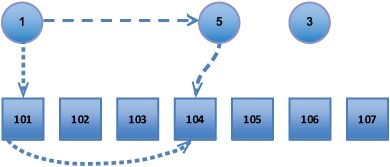
At the moment, the recommendations from the code in listing 4.3 are derived from a neighborhood of the 100 most similar users (NearestNUserNeighborhood was set to a neighborhood size of 100). The decision to use the 100 users whose similarity is greatest in order to make recommendations is arbitrary. What if this was 10? Recommendations would be based on fewer similar users but would exclude some less-similar users from consideration. See the visualization of a nearest-3 neighborhood in figure 4.1.
Figure 4.1. An illustration of defining a neighborhood of most similar users by picking a fixed number of closest neighbors. Here, distance illustrates similarity: farther means less similar. A neighborhood around user 1 is chosen to consist of the three most similar users: 5, 4, and 2.

Try replacing 100 with 10. The result of the evaluation, the average difference between estimated and actual preference values, is 0.98 or so. Recall that larger evaluation values are worse, so that’s a move in the wrong direction. The most likely explanation is that 10 users is too few. It’s likely that the eleventh and twelfth most similar users, and so on, add value. They’re still quite similar, and they’re associated with items that the first 10 most similar users weren’t.
Try a neighborhood of 500 users; the result drops to 0.75, which is of course better. You could evaluate many values and figure out the optimal setting for this data set, but the lesson is that there’s no magic value; some experimentation with real data is necessary to tune your recommender.
4.2.6. Threshold-based neighborhood
What if you don’t want to build a neighborhood of the n most similar users, but rather try to pick the pretty similar users and ignore everyone else? It’s possible to pick a similarity threshold and take any users that are at least that similar. Figure 4.2 illustrates a threshold-based definition of user neighborhood; contrast this with the fixed-size neighborhood in figure 4.1.
Figure 4.2. Defining a neighborhood of most-similar users with a similarity threshold

The threshold should be between –1 and 1, because all similarity metrics return similarity values in this range. At the moment, our example uses a standard Pearson correlation as the similarity metric. Those familiar with this correlation would likely agree that a value of 0.7 or above is a high correlation and constitutes a sensible definition of pretty similar. Let’s switch to use ThresholdUserNeighborhood. It’s as simple as changing one line to instead instantiate a ThresholdUserNeighborhood:
new ThresholdUserNeighborhood(0.7, similarity, model)
Now the evaluator scores the recommender at 0.84. What if the neighborhood were more selective, using a threshold of 0.9? The score worsens to 0.92; it’s likely that the same explanation applies as before—the neighborhood contains too few users at this threshold. How about 0.5? The score improves to 0.78. Examples that follow will use a threshold-based neighborhood with a threshold of 0.5.
Again, you’d likely want to explore many more values on real data to determine an optimum, but our simple experimentation has already improved estimation accuracy by about 15 percent.
4.3. Exploring similarity metrics
Another important part of user-based recommenders is the UserSimilarity implementation. A user-based recommender relies most of all on this component. Without a reliable and effective notion of which users are similar to others, this approach falls apart. The same is true of the user-based recommender’s cousin, the item-based recommender, which also relies on similarity. This component is so important that we spend almost a third of this chapter investigating standard similarity metrics and how they’re implemented in Mahout.
4.3.1. Pearson correlation–based similarity
So far, examples have used the PearsonCorrelationSimilarity implementation, which is a similarity metric based on the Pearson correlation.
The Pearson correlation is a number between –1 and 1 that measures the tendency of two series of numbers, paired up one-to-one, to move together. That is to say, it measures how likely a number in one series is to be relatively large when the corresponding number in the other series is high, and vice versa. It measures the tendency of the numbers to move together proportionally, such that there’s a roughly linear relationship between the values in one series and the other. When this tendency is high, the correlation is close to 1. When there appears to be little relationship at all, the value is near 0. When there appears to be an opposing relationship—one series’ numbers are high exactly when the other series’ numbers are low—the value is near –1.
Note
For statistically inclined readers, the Pearson correlation of two series is the ratio of their covariance to the product of their variances. Covariance is a measure of how much two series move together in absolute terms; it’s big when the series moves far in the same direction from their means in the same places. Dividing by the variances merely normalizes for the absolute size of their changes. It’s not essential to understand this and other alternative definitions in order to use the Pearson correlation within Mahout, but there’s lots of information on the web if you’re interested.
This concept, widely used in statistics, can be applied to users to measure their similarity. It measures the tendency of two users’ preference values to move together—to be relatively high, or relatively low, on the same items. For an example, let’s look again at the first sample data file we considered, intro.csv, as follows.
Listing 4.4. A simple recommender input file
1,101,5.0
1,102,3.0
1,103,2.5

2,101,2.0
2,102,2.5
2,103,5.0
2,104,2.0

3,101,2.5
3,104,4.0
3,105,4.5
3,107,5.0

4,101,5.0
4,103,3.0
4,104,4.5
4,106,4.0

5,101,4.0
5,102,3.0
5,103,2.0
5,104,4.0
5,105,3.5
5,106,4.0
We noted that users 1 and 5 seem similar because their preferences seem to run together. On items 101, 102, and 103, they roughly agree: 101 is the best, 102 somewhat less good, and 103 isn’t desirable. By the same reasoning, users 1 and 2 aren’t so similar. Note that our reasoning about user 1 can’t really include items 104 through 106, because user 1’s preferences for 104 through 106 aren’t known. The similarity computation can only operate on items that both users have expressed a preference for. (In section 4.3.9, we’ll look at what happens when missing preference values like this are inferred.)
The Pearson correlation captures these notions, as can be seen in table 4.1. The details of the computation aren’t reproduced here; refer to online sources such as http://www.socialresearchmethods.net/kb/statcorr.php for an explanation of how the correlation is computed.
Table 4.1. The Pearson correlation between user 1 and other users based on the three items that user 1 has in common with the others
|
Item 101 |
Item 102 |
Item 103 |
Correlation with user 1 |
|
|---|---|---|---|---|
| User 1 | 5.0 | 3.0 | 2.5 | 1.000 |
| User 2 | 2.0 | 2.5 | 5.0 | -0.764 |
| User 3 | 2.5 | - | - | - |
| User 4 | 5.0 | - | 3.0 | 1.000 |
| User 5 | 4.0 | 3.0 | 2.0 | 0.945 |
| Note A user’s Pearson correlation with itself is always 1.0. | ||||
4.3.2. Pearson correlation problems
Although the results are indeed intuitive, the Pearson correlation has some quirks in the context of recommender engines.
First, it doesn’t take into account the number of items in which two users’ preferences overlap, which is probably a weakness in the context of recommender engines. Two users that have seen 200 of the same movies, for instance, even if they don’t often agree on ratings, are probably more similar than two users who have only ever seen 2 movies in common. This issue appears in a small way in the preceding data; note that users 1 and 5 have both expressed preferences for all three items and seem to have similar tastes. Yet, users 1 and 4 have a higher correlation of 1.0, based on only two overlapping items. This seems a bit counterintuitive.
Second, if two users overlap on only one item, no correlation can be computed because of how the computation is defined. This is why no correlation can be computed between users 1 and 3. This could be an issue for small or sparse data sets, in which users’ item sets rarely overlap. Or, one could also view it as a benefit: two users who overlap for only one item are, intuitively, not very similar anyway.
Finally, the correlation is also undefined if either series of preference values are all identical. It doesn’t require that both series have all the same preference values. For example, if user 5 had expressed a preference of 3.0 for all three items, it wouldn’t be possible to compute a similarity between user 1 and user 5 because the Pearson correlation would be undefined, even though user 1 has preferences besides 3.0. This is likewise most probably an issue when users rarely overlap with others in the items they’ve expressed any preference for.
Although the Pearson correlation commonly appears in recommenders in early research papers,[1] and it appears in introductory books on recommenders, it isn’t necessarily a good first choice. It’s not necessarily bad, either; you simply need to understand how it works.
1 Appendix C lists some of these papers. See in particular Breese, Heckerman, and Kadie, “Empirical Analysis of Predictive Algorithms for Collaborative Filtering” and Herlocker, Konstan, Borchers, and Riedl, “An Algorithmic Framework for Performing Collaborative Filtering.”
4.3.3. Employing weighting
PearsonCorrelationSimilarity provides an extension to the standard computation, called weighting, that mitigates one of the preceding issues.
The Pearson correlation doesn’t reflect, directly, the number of items over which it’s computed, and for our purposes, that would be useful. When based on more information, the resulting correlation would be a more reliable result. In order to reflect this, it’s desirable to push positive correlation values toward 1.0 and negative values toward –1.0 when the correlation is based on more items. Alternatively, you could imagine pushing the correlation values towards some mean preference value when the correlation is based on fewer items; the effect would be similar, but the implementation would be somewhat more complex because it would require tracking the mean preference value for pairs of users.
In listing 4.3, passing the value Weighting.WEIGHTED to the constructor of PearsonCorrelationSimilarity as the second argument does this. It will cause the resulting correlation to be pushed towards 1.0, or –1.0, depending on how many data points were used to compute the correlation value. A quick rerun of the evaluation framework reveals that, in this case, this setting improves the score slightly to 0.77.
4.3.4. Defining similarity by Euclidean distance
Let’s try EuclideanDistanceSimilarity—swap in this implementation by changing the UserSimilarity implementation used in listing 4.3 to new EuclideanDistanceSimilarity(model) instead.
This implementation is based on the distance between users. This idea makes sense if you think of users as points in a space of many dimensions (as many dimensions as there are items), whose coordinates are preference values. This similarity metric computes the Euclidean distance d between two such user points.[2] This value alone doesn’t constitute a valid similarity metric, because larger values would mean more-distant, and therefore less similar, users. The value should be smaller when users are more similar. Therefore, the implementation actually returns 1 / (1+d). Refer to table 4.2, which illustrates this computation. You can verify that when the distance is 0 (users have identical preferences) the result is 1, decreasing to 0 as d increases. This similarity metric never returns a negative value, but larger values still mean more similarity.
2 Recall that the Euclidian distance is the square root of the sum of the squares of the differences in coordinates.
Table 4.2. The Euclidean distance between user 1 and other users, and the resulting similarity scores
|
Item 101 |
Item 102 |
Item 103 |
Distance |
Similarity to user 1 |
|
|---|---|---|---|---|---|
| User 1 | 5.0 | 3.0 | 2.5 | 0.000 | 1.000 |
| User 2 | 2.0 | 2.5 | 5.0 | 3.937 | 0.203 |
| User 3 | 2.5 | - | - | 2.500 | 0.286 |
| User 4 | 5.0 | - | 3.0 | 0.500 | 0.667 |
| User 5 | 4.0 | 3.0 | 2.0 | 1.118 | 0.472 |
After changing listing 4.3 to use EuclideanDistanceSimilarity, the result is 0.75—it happens to be a little better in this case, but barely. Note that some notion of similarity was computable for all pairs of users here, whereas the Pearson correlation couldn’t produce an answer for users 1 and 3. This is good, on the one hand, though the result is based on one item in common, which could be construed as undesirable. This implementation also has the same possibly counterintuitive behavior: users 1 and 4 have a higher similarity than users 1 and 5.
4.3.5. Adapting the cosine measure similarity
The cosine measure similarity is another similarity metric that depends on envisioning user preferences as points in space. Hold in mind the image of user preferences as points in an n-dimensional space. Now imagine two lines from the origin, or point (0,0,...,0), to each of these two points. When two users are similar, they’ll have similar ratings, and so will be relatively close in space—at least, they’ll be in roughly the same direction from the origin. The angle formed between these two lines will be relatively small. In contrast, when the two users are dissimilar, their points will be distant, and likely in different directions from the origin, forming a wide angle.
This angle can be used as the basis for a similarity metric in the same way that the Euclidean distance was used to form a similarity metric. In this case, the cosine of the angle leads to a similarity value. If you’re rusty on trigonometry, all you need to remember to understand this is that the cosine value is always between –1 and 1: the cosine of a small angle is near 1, and the cosine of a large angle near 180 degrees is close to –1. This is good, because small angles should map to high similarity, near 1, and large angles should map to near –1.
You may be searching for something like CosineMeasureSimilarity in Mahout, but you’ve already found it, under an unexpected name: PearsonCorrelationSimilarity. The cosine measure similarity and Pearson correlation aren’t the same thing, but if you bother to work out the math, you’ll discover that they actually reduce to the same computation when the two series of input values each have a mean of 0 (centered). The Mahout implementation centers the input, so the two are the same.
The cosine measure similarity is commonly referenced in research on collaborative filtering. You can employ this similarity metric by simply using PearsonCorrelationSimilarity.
4.3.6. Defining similarity by relative rank with the Spearman correlation
The Spearman correlation is an interesting variant on the Pearson correlation, for our purposes. Rather than compute a correlation based on the original preference values, it computes a correlation based on the relative rank of preference values. Imagine that, for each user, their least-preferred item’s preference value is overwritten with a 1. Then the next-least-preferred item’s preference value is changed to 2, and so on. To illustrate this, imagine that you were rating movies and gave your least-preferred movie one star, the next-least favorite two stars, and so on. Then, a Pearson correlation is computed on the transformed values. This is the Spearman correlation.
This process loses some information. Although it preserves the essence of the preference values—their ordering—it removes information about exactly how much more each item was liked than the last. This may or may not be a good idea; it’s somewhere between keeping preference values and forgetting them entirely—two possibilities that we’ve explored before.
Table 4.3 shows the resulting Spearman correlations. Its simplifications on this already-simple data set result in some extreme values: in fact, all correlations are 1 or –1 here, depending on whether a user’s preference values run with or counter to user 1’s preferences. As with the Pearson correlation, no value can be computed between users 1 and 3.
Table 4.3. The preference values transformed into ranks, and the resulting Spearman correlation between user 1 and each of the other users
|
Item 101 |
Item 102 |
Item 103 |
Correlation to user 1 |
|
|---|---|---|---|---|
| User 1 | 3.0 | 2.0 | 1.0 | 1.0 |
| User 2 | 1.0 | 2.0 | 3.0 | –1.0 |
| User 3 | 1.0 | - | - | - |
| User 4 | 2.0 | - | 1.0 | 1.0 |
| User 5 | 3.0 | 2.0 | 1.0 | 1.0 |
SpearmanCorrelationSimilarity implements this idea. You could try using this as the UserSimilarity in the evaluator code from before. Run it, and take a long coffee break. Turn in for the night. It won’t finish anytime soon. This implementation is far slower because it must do some nontrivial work to compute and store these ranks. The Spearman correlation–based similarity metric is expensive to compute, and is therefore possibly more of academic interest than practical use. For some small data sets, though, it may be desirable.
This is a fine time to introduce one of many caching wrapper implementations available in Mahout. CachingUserSimilarity is a UserSimilarity implementation that wraps another UserSimilarity implementation and caches its results. That is, it delegates computation to another, given implementation, and remembers those results internally. Later, when it’s asked for a user-user similarity value that was previously computed, it can answer immediately rather than ask the given implementation to compute it again. In this way, you can add caching to any similarity implementation. When the cost of performing a computation is relatively high, as here, it can be worthwhile to employ. The cost, of course, is the memory consumed by the cache.
Instead of just using SpearmanCorrelationSimilarity, try using the implementation shown in the following listing.
Listing 4.5. Employing caching with a UserSimilarity implementation
UserSimilarity similarity = new CachingUserSimilarity(
    new SpearmanCorrelationSimilarity(model), model);
It’s also advisable to decrease the amount of test data from 5 percent to 1 percent by increasing the trainingPercentage argument to evaluate() from 0.95 to 0.99. It would also be wise to decrease the evaluation percentage from 5 percent to 1 percent by changing the last parameter from 0.05 to 0.01. This will allow the evaluation to finish in more like tens of minutes.
The result should be near 0.80. Again, broad conclusions are difficult to draw: on this particular data set, it was not quite as effective as other similarity metrics.
4.3.7. Ignoring preference values in similarity with the Tanimoto coefficient
Interestingly, there are also UserSimilarity implementations that ignore preference values entirely. They don’t care whether a user expresses a high or low preference for an item—only that the user expresses a preference at all. As we discussed in chapter 3, it doesn’t necessarily hurt to ignore preference values.
TanimotoCoefficientSimilarity is one such implementation, based on (surprise) the Tanimoto coefficient. This value is also known as the Jaccard coefficient. It’s the number of items that two users express some preference for, divided by the number of items that either user expresses some preference for, as illustrated in figure 4.3.
Figure 4.3. The Tanimoto coefficient is the ratio of the size of the intersection, or overlap, in two users’ preferred items (the dark area), to the union of the users’ preferred items (the dark and light areas together).

In other words, it’s the ratio of the size of the intersection to the size of the union of their preferred items. It has the required properties: when two users’ items completely overlap, the result is 1.0. When they have nothing in common, it’s 0.0. The value is never negative, but that’s OK. It’s possible to expand the results into the range –1 to 1 with some simple math: similarity = 2 • similarity – 1. It won’t matter to the framework.
Table 4.4 shows the value of the Tanimoto coefficient similarity between user 1 and other users.
Table 4.4. The similarity values between user 1 and other users, computed using the Tanimoto coefficient. Note that preference values themselves are omitted, because they aren’t used in the computation.
|
Item 101 |
Item 102 |
Item 103 |
Item 104 |
Item 105 |
Item 106 |
Item 107 |
Similarity to user 1 |
|
|---|---|---|---|---|---|---|---|---|
| User 1 | X | X | X | 1.0 | ||||
| User 2 | X | X | X | X | 0.75 | |||
| User 3 | X | X | X | X | 0.17 | |||
| User 4 | X | X | X | X | 0.4 | |||
| User 5 | X | X | X | X | X | X | 0.5 |
Note that this similarity metric doesn’t depend only on the items that both users have some preference for, but that either user has some preference for. Hence, all seven items appear in the calculation, unlike before.
You’re likely to use this similarity metric if, and only if, your underlying data contains only Boolean preferences and you have no preference values to begin with. If you do have preference values, you might use this metric because you believe there’s more signal than noise in the values. You would usually do better with a metric that uses the preference information. In the GroupLens data set, using the Tanimoto coefficient gives a slightly worse score of 0.82.
4.3.8. Computing smarter similarity with a log-likelihood test
Log-likelihood–based similarity is similar to the Tanimoto coefficient–based similarity, though it’s more difficult to understand intuitively. It’s another metric that doesn’t take account of individual preference values. The math involved in computing this similarity metric is beyond the scope of this book to explain. Like the Tanimoto coefficient, it’s based on the number of items in common between two users, but its value is more an expression of how unlikely it is for two users to have so much overlap, given the total number of items out there and the number of items each user has a preference for.
To illustrate, consider two movie fans who have each seen and rated several movies but have only both seen Star Wars and Casablanca. Are they similar? If they’ve each seen hundreds of movies, it wouldn’t mean much. Many people have seen these movies, and if these two have seen many movies but only managed to overlap in these two, they’re probably not similar. On the other hand, if each user has seen just a few movies, and these two were on both users’ lists, it would seem to imply that they’re similar people when it comes to movies; the overlap would be significant.
The Tanimoto coefficient already encapsulates some of this thinking, because it looks at the ratio of the size of the intersection of their interests to the union. The log-likelihood is computing something slightly different. It’s trying to assess how unlikely it is that the overlap between the two users is just due to chance. That is to say, two dissimilar users will no doubt happen to rate a couple movies in common, but two similar users will show an overlap that looks quite unlikely to be mere chance. With some statistical tests, this similarity metric attempts to determine just how strongly unlikely it is that two users have no resemblance in their tastes; the more unlikely, the more similar the two should be. The resulting similarity value may be interpreted as a probability that the overlap isn’t due to chance.
These similarity values are shown for our small data set in table 4.5. As you can see, user 1’s similarity with user 1, or any other user with identical preferred items, isn’t 1.0 under this measure. Using a log-likelihood–based similarity metric is as easy as inserting new LogLikelihoodSimilarity in listing 4.3, as before.
Table 4.5. The similarity values between user 1 and other users, computed using the log-likelihood similarity metric
|
Item 101 |
Item 102 |
Item 103 |
Item 104 |
Item 105 |
Item 106 |
Item 107 |
Similarity to user 1 |
|
|---|---|---|---|---|---|---|---|---|
| User 1 | X | X | X | 0.90 | ||||
| User 2 | X | X | X | X | 0.84 | |||
| User 3 | X | X | X | X | 0.55 | |||
| User 4 | X | X | X | X | 0.16 | |||
| User 5 | X | X | X | X | X | X | 0.55 |
Although it’s hard to generalize, log-likelihood–based similarity will probably outperform Tanimoto coefficient–based similarity. It is, in a sense, a more intelligent metric. Rerunning the evaluation shows that, at least for this data set and recommender, it improves performance over TanimotoCoefficientSimilarity, to 0.73.
4.3.9. Inferring preferences
Sometimes too little data is a problem. In a few cases, for example, the Pearson correlation was unable to compute any similarity value at all because some pairs of users overlap in only one item. The Pearson correlation also can’t take account of preference values for items for which only one user has expressed a preference.
What if a default value were filled in for all the missing data points? For example, the framework could pretend that each user has rated every item by inferring preferences for items for which the user hasn’t explicitly expressed a preference. This sort of strategy is enabled via the PreferenceInferrer interface, which currently has one implementation, AveragingPreferenceInferrer. This implementation computes the average preference value for each user and fills in this average as the preference value for any item not already associated with the user. It can be enabled on a UserSimilarity implementation with a call to setPreferenceInferrer().
Although this strategy is available, it’s not usually helpful in practice. It’s provided primarily because it’s mentioned in early research papers on recommender engines. In theory, making up information purely based on existing information isn’t adding anything, but it certainly does slow down computations drastically. It’s available for experimentation but will likely not be useful when applied to real data sets.
You’ve now seen all of the user-user similarity metrics that are implemented within Mahout. This knowledge pays double dividends, because the very same implementations in Mahout also provide an analogous notion of item-item similarity. That is, the same computations can be applied to define how similar items are, not just users. This is just in time, because the notion of similarity is likewise the basis of the next style of Mahout recommender implementation you’ll meet, the item-based recommender.
4.4. Item-based recommendation
We’ve looked at user-based recommenders in Mahout—not one recommender, but tools to build a nearly limitless number of variations on the basic user-based approach, by plugging different and differently configured components into the implementation.
It’s natural to look next at item-based recommenders. This section will be shorter, because several of the components in the preceding discussion (data models, similarity implementations) also apply to item-based recommenders.
Item-based recommendation is derived from how similar items are to items, instead of users to users. In Mahout, this means they’re based on an ItemSimilarity implementation instead of UserSimilarity. To illustrate, let’s return to the pair we left in the music store, doing their best to pick an album that a teenage boy would like. Imagine yet another line of reasoning they could have adopted:
| ADULT: | I’m looking for a CD for a teenage boy. |
| EMPLOYEE: | What kind of music or bands does he like? |
| ADULT: | He wears a Bowling In Hades T-shirt all the time and seems to have all of their albums. Anything else you’d recommend? |
| EMPLOYEE: | Well, about everyone I know that likes Bowling In Hades seems to like the new Rock Mobster album. |
This sounds reasonable. It’s different from previous examples, too. The record store employee is recommending an item that’s similar to something they already know the boy likes. This isn’t the same as before, where the question was, “Who is similar to the boy, and what do they like?” Here the question is, “What is similar to what the boy likes?”
Figure 4.4 attempts to illustrate this difference, which is the essential difference between user-based and item-based recommenders. They go by different paths to find recommended items: via similar users, and via similar items, respectively.
Figure 4.4. A basic illustration of the difference between user-based and item-based recommendation: user-based recommendation (large dashes) finds similar users, and sees what they like. Item-based recommendation (short dashes) sees what the user likes, and then finds similar items.
4.4.1. The algorithm
The algorithm will feel familiar to you since you have seen user-based recommenders already. This is also how the algorithm is implemented in Mahout.
for every item i that u has no preference for yet
  for every item j that u has a preference for
    compute a similarity s between i and j
    add u's preference for j, weighted by s, to a running average
return the top items, ranked by weighted average
The third line shows how it’s based on item-item similarities, not user-user similarities as before. The algorithms are similar, but not entirely symmetric. They do have notably different properties. For instance, the running time of an item-based recommender scales up as the number of items increases, whereas a user-based recommender’s running time goes up as the number of users increases.
This suggests one reason that you might choose an item-based recommender: if the number of items is relatively low compared to the number of users, the performance advantage could be significant.
Also, items are typically less subject to change than users. When items are things like DVDs, it’s reasonable to expect that over time, as you acquire more data, estimates of the similarities between items converge. There is no reason to expect them to change radically or frequently. Some of the same may be said of users, but users can change over time and new knowledge of users is likely to come in bursts of new information that must be digested quickly. To connect this to the last example, it’s likely that Bowling In Hades albums and Rock Mobster albums will remain as similar to each other next year as today. But it’s a lot less likely that the same fans mentioned above will have the same tastes next year, and so their similarities will change more.
If item-item similarities are more fixed, they’re better candidates for precomputation. Precomputing similarities takes work, but it speeds up recommendations at runtime. This could be desirable in contexts where delivering recommendations quickly at runtime is essential—think about a news site that must potentially deliver recommendations immediately with each news article view.
In Mahout, the GenericItemSimilarity class can be used to precompute and store the results from any ItemSimilarity. It can be applied to any of the implementations you have seen, and can be added to the code snippets that follow, if you wish.
4.4.2. Exploring the item-based recommender
Let’s insert a simple item-based recommender into our familiar evaluation framework, using the following code. It deploys a GenericItemBasedRecommender rather than GenericUserBasedRecommender, and it requires a different and simpler set of dependencies.
Listing 4.6. The core of a basic item-based recommender
public Recommender buildRecommender(DataModel model)
    throws TasteException {
  ItemSimilarity similarity = new PearsonCorrelationSimilarity(model);
  return new GenericItemBasedRecommender(model, similarity);
}
PearsonCorrelationSimilarity still works here because it also implements the ItemSimilarity interface, which is entirely analogous to the UserSimilarity interface. It implements the same notion of similarity, based on the Pearson correlation, but between items instead of users. That is, it compares series of preferences expressed by many users, for one item, rather than by one user for many items.
GenericItemBasedRecommender is simpler. It only needs a DataModel and ItemSimilarity—there’s no ItemNeighborhood. You might wonder at the apparent asymmetry. Recall that the item-based recommendation process already begins with a limited number of starting points: the items that the user in question already expresses a preference for. This is analogous to the neighborhood of similar users that the user-based approach first identifies. It doesn’t make sense in the second half of the algorithm to compute neighborhoods around each of the user’s preferred items.
You’re invited to experiment with different similarity metrics, as we did for users. Not all of the implementations of UserSimilarity also implement ItemSimilarity. You already know how to evaluate the accuracy of this item-based recommender when using various similarity metrics on the now-familiar GroupLens data set. The results are reproduced for convenience in table 4.6.
Table 4.6. Evaluation results under various ItemSimilarity metrics
|
Implementation |
Similarity |
|---|---|
| PearsonCorrelationSimilarity | 0.75 |
| PearsonCorrelationSimilarity + weighting | 0.75 |
| EuclideanDistanceSimilarity | 0.76 |
| EuclideanDistanceSimilarity + weighting | 0.78 |
| TanimotoCoefficientSimilarity | 0.77 |
| LogLikelihoodSimilarity | 0.77 |
One thing you may notice is that this recommender setup runs significantly faster. That’s not surprising, given that the data set has about 70,000 users and 10,000 items. Item-based recommenders are generally faster when there are fewer items than users. You may, as a result, wish to increase the percentage of data used in the evaluation to 20 percent or so (pass 0.2 as the final argument to evaluate()). This should result in a more reliable evaluation. Note that there’s little apparent difference among these implementations on this data set.
4.5. Slope-one recommender
Did you like the movie Carlito’s Way? Most people who liked this movie, it seems, also liked another film starring Al Pacino, Scarface. But people tend to like Scarface a bit more. We’d imagine most people who think of Carlito’s Way as a four-star movie would give Scarface five stars. So if you told us you thought Carlito’s Way was a three-star movie, we might guess you’d give Scarface four stars—one more than the other film.
If you agree with this sort of reasoning, you’ll like the slope-one recommender (http://en.wikipedia.org/wiki/Slope_One). It estimates preferences for new items based on average difference in the preference value (diffs) between a new item and the other items the user prefers.
For example, let’s say that, on average, people rate Scarface higher by 1.0 than Carlito’s Way. Let’s also say that everyone rates Scarface the same as The Godfather, on average. And now, there’s a user who rates Carlito’s Way as 2.0, and The Godfather as 4.0. What’s a good estimate of their preference for Scarface?
Based on Carlito’s Way, a good guess would be 2.0 + 1.0 = 3.0. Based on The Godfather, it might be 4.0 + 0.0 = 4.0. A better guess still might be the average of the two: 3.5. This is the essence of the slope-one recommender approach.
4.5.1. The algorithm
The slope-one name comes from the fact that the recommender algorithm starts with the assumption that there’s some linear relationship between the preference values for one item and another, that it’s valid to estimate the preferences for some item Y based on the preferences for item X, via some linear function like Y = mX + b. Then the slope-one recommender makes the additional simplifying assumption that m = 1: slope one. It just remains to find b = Y - X, the (average) difference in preference value, for every pair of items.
This means the algorithm consists of a significant preprocessing phase, in which all item-item preference value differences are computed:
for every item i
  for every other item j
    for every user u expressing preference for both i and j
      add the difference in u's preference for i and j to an average
And then, the recommendation algorithm looks like this:
for every item i the user u expresses no preference for
  for every item j that user u expresses a preference for
    find the average preference difference between j and i
    add this diff to u's preference value for j
    add this to a running average
return the top items, ranked by these averages
The average diffs over the small sample recommender inputs from several prior examples in the book are shown in table 4.7.
Table 4.7. Average differences in preference values between all pairs of items. Cells along the diagonal are 0.0. Cells in the bottom left are simply the negative of their counterparts across the diagonal, so these aren’t represented explicitly. Some diffs don’t exist, such as 102-107, because no user expressed a preference for both 102 and 107.
|
Item 101 |
Item 102 |
Item 103 |
Item 104 |
Item 105 |
Item 106 |
Item 107 |
|
|---|---|---|---|---|---|---|---|
| Item 101 | –0.833 | 0.875 | 0.25 | 0.75 | –0.5 | 2.5 | |
| Item 102 | 0.333 | 0.25 | 0.5 | 1.0 | - | ||
| Item 103 | 0.167 | 1.5 | 1.5 | - | |||
| Item 104 | 0.0 | –0.25 | 1.0 | ||||
| Item 105 | 0.5 | 0.5 | |||||
| Item 106 | - | ||||||
| Item 107 |
Slope-one is attractive because the online portion of the algorithm is fast. Like an item-based recommender, its performance doesn’t depend upon the number of users in the data model. It depends only upon the average preference difference between every pair of items, which can be precomputed. Further, its underlying data structure can be efficiently updated: when a preference changes, it’s simple to update the relevant diff values. In contexts where preferences may change quickly, this is an asset.
Note that the memory requirements necessary to store all of these item-item differences in preference values grow as the square of the number of items. Twice as many items means four times the memory!
4.5.2. Slope-one in practice
You can easily try the slope-one recommender. It takes no similarity metric as a necessary argument:
new SlopeOneRecommender(model)
After running a standard evaluation using, again, the GroupLens 10 million rating data set, you’ll get a result near 0.65. That’s the best yet. Indeed, the simple slope-one approach works well in many cases. This algorithm doesn’t make use of a similarity metric, unlike the other approaches so far. It has relatively few knobs to twiddle.
Like the Pearson correlation, the simplest form of the slope-one algorithm has a vulnerability: item-item diffs are given equal weighting regardless of how reliable they are—how much data they’re based upon. Let’s say only one user in the history of movie watching has rated both Carlito’s Way and The Notebook. It’s possible; they’re quite different films. It’s easy to compute a diff for these two films, but would it be as useful as the diff between Carlito’s Way and The Godfather, which are averaged over thousands of users? It sounds unlikely. The latter diff is probably more reliable because it’s an average over a higher number of users.
Again, some form of weighting may help to improve these recommendations. SlopeOneRecommender offers two types of weighting: weighting based on count and on standard deviation. Recall that slope-one estimates the preference values by adding diffs to all of the user’s current preference values and then averaging all of those results together to form an estimate. Count weighting will weight more heavily those diffs that are based on more data. The average becomes a weighted average, where the diff count is the weight—the number of users on which the diff is based.
Similarly, standard deviation weighting will weight according to the standard deviation of difference in preference value. A lower standard deviation means a higher weighting. If the difference in preference value between two films is very consistent across many users, it seems more reliable and should be given more weight. If it varies considerably from user to user, it should be deemphasized.
These variants turn out to be enough of a good idea that they’re enabled by default. You already used this strategy when you ran the previous evaluation. Disable them to see the effect, as follows.
Listing 4.7. Selecting no weighting with a SlopeOneRecommender
DiffStorage diffStorage = new MemoryDiffStorage(
    model, Weighting.UNWEIGHTED, Long.MAX_VALUE));
return new SlopeOneRecommender(
 model,
 Weighting.UNWEIGHTED,
 Weighting.UNWEIGHTED,
 diffStorage);
The result is 0.67—only slightly worse on this data set.
4.5.3. DiffStorage and memory considerations
Slope-one does have its price: memory consumption. In fact, if you tweak the evaluation to use just 10 percent of all data (about 100,000 ratings), even a gigabyte of heap space won’t be enough. The diffs are used so frequently, and it’s so relatively expensive to compute them, that they do need to be computed and stored ahead of time. But keeping them all in memory can get expensive. It may become necessary to store diffs elsewhere.
Fortunately, implementations like MySQLJDBCDiffStorage exist for this purpose, allowing diffs to be computed and updated from a database. It must be used in conjunction with a JDBC-backed DataModel implementation like MySQLJDBCDataModel, as shown in the next listing.
Listing 4.8. Creating a JDBC-backed DiffStorage
AbstractJDBCDataModel model = new MySQLJDBCDataModel();
DiffStorage diffStorage = new MySQLJDBCDiffStorage(model);
Recommender recommender = new SlopeOneRecommender(
    model, Weighting.WEIGHTED, Weighting.WEIGHTED, diffStorage);
As with MySQLJDBCDataModel, the table name and column names used by MySQLJDBCDiffStorage can be customized via constructor parameters.
4.5.4. Distributing the precomputation
Precomputing the item-item diffs is significant work. Although it’s more likely that the size of your data will cause problems with memory requirements before the time required to compute these diffs becomes problematic, you might be wondering if there are ways to distribute this computation to complete it faster. Diffs can be updated easily at runtime in response to new information, so a relatively infrequent offline precomputation process is feasible in this model.
Distributing the diff computation via Hadoop is supported. Chapter 6 will introduce all of the Hadoop-related recommender support in Mahout, to explore this process.
4.6. New and experimental recommenders
Mahout also contains implementations of other approaches to recommendation. The three implementations presented briefly in this section are newer: the implementations may still be evolving, or the technique may be more recent and experimental. All are worthy ideas that may be useful for use or for modification.
4.6.1. Singular value decomposition–based recommenders
Among the most intriguing of these implementations is SVDRecommender, based on the singular value decomposition (SVD). This is an important technique in linear algebra that pops up in machine learning techniques. Fully understanding it requires some advanced matrix math and understanding of matrix factorization, but this isn’t necessary to appreciate SVD’s application to recommenders.
To outline the intuition behind what SVD does for recommenders, let’s say you ask a friend what sort of music she likes, and she lists the following artists:
- Brahms
- Chopin
- Miles Davis
- Tchaikovsky
- Louis Armstrong
- Schumann
- John Coltrane
- Charlie Parker
She might as well have summarized that she likes classical and jazz music. That communicates less precise information, but not a great deal less. From either statement, you could (probably correctly) infer that she would appreciate Beethoven more than the classic rock band Deep Purple.
Of course, recommender engines operate in a world of many specific data points, not generalities. The input is user preferences for a lot of particular items—more like the preceding list than this summary. It would be nice to operate on a smaller set of data, all else equal, for reasons of performance. If, for example, iTunes could base its Genius recommendations not on billions of individual song ratings, but instead on millions of ratings of genres, it would be faster—and, as a basis for recommending music, it might not be much worse.
Here, SVD is the magic that can do the equivalent of the preceding summarization. It boils down the world of user preferences for individual items to a world of user preferences for more general and less numerous features (like genre). This is, potentially, a much smaller set of data.
Although this process loses some information, it can sometimes improve recommendation results. The process smooths the input in useful ways. For example, imagine two car enthusiasts. One loves Corvettes, and the other loves Camaros, and they want car recommendations. These enthusiasts have similar tastes: both love a Chevrolet sports car. But in a typical data model for this problem, these two cars would be different items. Without any overlap in their preferences, these two users would be deemed unrelated. However, an SVD-based recommender would perhaps find the similarity. The SVD output may contain features that correspond to concepts like Chevrolet or sports car, with which both users would be associated. From the overlap in features, a similarity could be computed.
Using the SVDRecommender is as simple as this:
new SVDRecommender(model, new ALSWRFactorizer(model, 10, 0.05, 10))
SVDRecommender uses a Factorizer to perform its work; a fine first choice is the ALSWRFactorizer implementation used here. We won’t discuss your choices of Factorizer in detail here.
The first numeric argument is the number of features that the SVD should target. There’s no right answer for this; it would be equivalent to the number of genres that you condensed someone’s musical taste into, in this section’s first example. The second argument is lambda and it controls a feature of the factorizer called regularization. The last argument is the number of training steps to run. Think of this as controlling the amount of time it should spend producing this summary; larger values mean longer training.
This approach can give good results (0.69 on the GroupLens data set). At the moment, the major issue with the implementation is that it computes the SVD in memory. This requires the entire data set to fit in memory, and it’s precisely when this isn’t the case that this technique is appealing, because it can shrink the input without compromising output quality significantly. In the future, this algorithm will be reimplemented in terms of Hadoop, so the necessarily massive SVD computation can be distributed across multiple machines. It isn’t yet available at this stage of Mahout’s evolution.
4.6.2. Linear interpolation item–based recommendation
Linear interpolation is a somewhat different take on item-based recommendation, implemented as KnnItemBasedRecommender. Knn is short for k nearest neighbors, which is an idea also embodied in NearestNUserNeighborhood. As you saw earlier in figure 4.1, a UserNeighborhood implementation selects a fixed number of most similar users as a neighborhood of similar users. This linear interpolation algorithm uses the concept of a user neighborhood, but in a different way.
KnnItemBasedRecommender still estimates preference values by means of a weighted average of the items the user already has a preference for, but the weights aren’t the results of a similarity metric. Instead, the algorithm calculates the optimal set of weights to use between all pairs of items by means of some linear algebra—here’s where the linear interpolation comes in. Yes, it’s possible to optimize the weights with some mathematical wizardry.
In reality, it would be very expensive to compute this across all pairs of items, so instead it first calculates a neighborhood of items most similar to the target item—the item for which a preference is being estimated. It chooses the n nearest neighbors, in much the same way that NearestNUserNeighborhood did. One can try KnnItemBasedRecommender as shown in the following listing.
Listing 4.9. Deploying KnnItemBasedRecommender
ItemSimilarity similarity = new LogLikelihoodSimilarity(model);
Optimizer optimizer = new NonNegativeQuadraticOptimizer();
return new KnnItemBasedRecommender(model, similarity, optimizer, 10);
This code will cause the recommender to use a log-likelihood similarity metric to calculate nearest-10 neighborhoods of items. Then it’ll use a quadratic programming–based strategy to calculate the linear interpolation. The details of this calculation are outside the scope of the book.
The implementation is quite functional, but in its current form, it’s also slow on moderately sized data sets. It should be viewed as viable for small data sets, or for study and extension. On the GroupLens data set, it yields an evaluation result of 0.76.
4.6.3. Cluster-based recommendation
Cluster-based recommendation is best thought of as a variant on user-based recommendation. Instead of recommending items to users, items are recommended to clusters of similar users. This entails a preprocessing phase, in which all users are partitioned into clusters. Recommendations are then produced for each cluster, such that the recommended items are most interesting to the largest number of users.
The upside of this approach is that recommendation is fast at runtime because almost everything is precomputed. One could argue that the recommendations are less personal this way, because recommendations are computed for a group rather than an individual. This approach may be more effective at producing recommendations for new users, who have little preference data available. As long as the user can be attached to a reasonably relevant cluster, the recommendations ought to be as good as they’ll be when more is known about the user.
The name comes from the fact that the algorithm repeatedly joins most-similar clusters into larger clusters, and this implicitly organizes users into a sort of hierarchy, or tree, as depicted in figure 4.5.
Figure 4.5. An illustration of clustering. Users 1 and 5 are clustered together first, as are 2 and 3, because they’re closest. Then, 4 is clustered with the 1-5 cluster to create a larger cluster, one step up in the “tree.”

Unfortunately, the clustering takes a long time, as you’ll see if you attempt to run the code in the following listing, which employs a TreeClusteringRecommender to implement this idea.
Listing 4.10. Creating a cluster-based recommender
UserSimilarity similarity = new LogLikelihoodSimilarity(model);
ClusterSimilarity clusterSimilarity =
    new FarthestNeighborClusterSimilarity(similarity);
return new TreeClusteringRecommender(model, clusterSimilarity, 10);
Similarity between users is, as usual, defined by a UserSimilarity implementation. Similarity between two clusters of users is defined by a ClusterSimilarity implementation. Currently, two implementations are available: one defines cluster similarity as the similarity between the two most similar user pairs, one chosen from each cluster; the other defines cluster similarity as the similarity between the two least similar users.
Both approaches are reasonable; in both cases the risk is that one outlier on the edge of a cluster distorts the notion of cluster similarity. Two clusters whose members are on average distant but happen to be close at one edge would be considered quite close by the most-similar-user rule, which is implemented by NearestNeighborClusterSimilarity. The least-similar-user rule, implemented by FarthestNeighborClusterSimilarity in listing 4.10, likewise may consider two fairly close clusters to be distant from one another if each contains an outlier far away from the opposite cluster.
A third approach, defining cluster similarity as the distance between the centers, or means, of two clusters, is also possible, though not yet implemented in this part of Mahout.
4.7. Comparison to other recommenders
As mentioned earlier in the book, content-based recommendation is a broad and often-mentioned approach to recommendation that takes into account the content or attributes of items. For this reason, it’s similar to, yet distinct from, collaborative filtering approaches, which are based on user associations with items only, and treats items as black boxes without attributes. Although Mahout largely doesn’t implement content-based approaches, it does offer some opportunities to make use of item attributes in recommendation computations.
4.7.1. Injecting content-based techniques into Mahout
For example, consider an online bookseller who stocks multiple editions of some books. This seller might recommend books to its customers. Its items are books, of course, and it might naturally define a book by its ISBN number (a unique product identifier). But for a popular public-domain book like Jane Eyre, there may be many printings by different publishers of the same text, under different ISBN numbers. It seems more natural to recommend books based on their texts, rather than on a particular edition—do you care more about reading “Jane Eyre” or “Jane Eyre as printed by ACME Publications in 1993 in paperback?” Rather than treat various publications of Jane Eyre as distinct items, it might be more useful to think of the book itself, the text, as the item, and recommend all editions of this book equally. This would be, in a sense, content-based recommendation. By treating the underlying text of a book product, which is its dominant attribute, as the item in a collaborative filtering sense, and then applying collaborative filtering techniques with Mahout, the seller would be engaging in a form of content-based recommendation.
Or recall that item-based recommenders require some notion of similarity between two given items. This similarity is encapsulated by an ItemSimilarity implementation. So far, implementations have derived similarity from user preferences only—this is classic collaborative filtering. But there’s no reason the implementation couldn’t be based on item attributes. For example, a movie recommender might define item (movie) similarity as a function of movie attributes like genre, director, actor, and year of release. Using such an implementation within a traditional item-based recommender would also be an example of content-based recommendation.
4.7.2. Looking deeper into content-based recommendation
Taking this a step further, imagine content-based recommendation as a generalization of collaborative filtering. In collaborative filtering, computations are based on preferences, which are user-item associations. But what drives these user-item associations? It’s likely that users have implicit preferences for certain item attributes, which come out in their preferences for certain items and not others. For example, if your friend told you she likes the albums Led Zeppelin I, Led Zeppelin II, and Led Zeppelin III, you might well guess she is actually expressing a preference for an attribute of these items: the band Led Zeppelin. By discovering these associations, and discovering attributes of items, it’s possible to construct recommender engines based on these more nuanced understandings of user-item associations.
These techniques come to resemble search and document-retrieval techniques: asking what items a user might like based on user-attribute associations and item attributes resembles retrieving search results based on query terms and the occurrence of terms in documents. Although Mahout’s recommender support doesn’t yet embrace these techniques, it’s a natural direction for future versions to address.
4.8. Comparison to model-based recommenders
Another future direction for Mahout is model-based recommendation. This family of techniques attempts to build some model of user preferences based on existing preferences, and then infer new preferences. These techniques generally fall into the broader category of collaborative filtering, because they typically derive from user preferences only.
The model might be a probabilistic picture of users’ preferences, in the form of a Bayesian network, for example. The algorithm then attempts to judge the probability of liking an item given its knowledge of all user preferences, and it ranks the recommendations accordingly.
Association rule learning can be applied in a similar sense to recommendations. By learning rules such as “when a user prefers item X and item Y, they will prefer item Z” from the data, and judging confidence in the reliability of such rules, a recommender can put together the most likely set of new, preferred items.
Cluster-based recommenders might be considered a type of model-based recommender. The clusters represent a model of how users group together and therefore how their preferences might run the same way. In this limited sense, Mahout supports model-based recommenders. But this is an area that’s still largely under construction in Mahout as of this writing.
4.9. Summary
In this chapter, we thoroughly explored the core recommender algorithms offered by Mahout.
We started by explaining the general user-based recommender algorithm in terms of real-world reasoning. From there, we looked at how this algorithm is realized in Mahout, as GenericUserBasedRecommender. Many pieces of this generic approach can be customized, such as the definition of user similarity and user neighborhood.
We looked at the classic user similarity metric, based on the Pearson correlation, noted some possible issues with this approach, and looked at responses such as weighting. We looked at similarity metrics based on the Euclidean distance, Spearman correlation, Tanimoto coefficient, and log-likelihood ratio.
Then we examined another canonical recommendation technique, item-based recommendation, as implemented by GenericItemBasedRecommender. It reuses some concepts already covered in the context of user-based recommenders, such as the Pearson correlation.
Next, we examined a slope-one recommender, a unique and relatively simple approach to recommendation based on average differences in preference values between items. It requires significant precomputation and storage for these diffs, so we explored how to store these both in memory and in a database.
Last, we looked briefly at a few newer, more experimental implementations currently in the framework. These include implementations based on singular value decomposition, linear interpolation, and clustering. These may be useful for small data sets, or may be of academic interest, because they’re still a work in progress.
The key parameters and features for each implementation are summarized in table 4.8.
Table 4.8. Summary of available recommender implementations in Mahout, their key input parameters, and key features to consider when choosing an implementation
|
Implementation |
Key parameters |
Key features |
|---|---|---|
| GenericUserBasedRecommender |
|
|
| GenericItemBasedRecommender |
|
|
| SlopeOneRecommender |
|
|
| SVDRecommender |
|
|
| KnnItemBasedRecommender |
|
|
| TreeClusteringRecommender |
|
|
We’re done introducing Mahout’s recommender engine support. Now we’re ready to examine even larger and more realistic data sets, from the practitioner’s perspective. You might wonder why we’ve made little mention of Hadoop yet. Hadoop is a powerful tool, and it’s necessary when dealing with massive data sets, where one must make use of many machines. This has drawbacks: such computations are massive, they’re resource-intensive, and they complete in hours, not milliseconds. We’ll reach Hadoop in the last chapter in this section.
First, in the next chapter, we create a production-ready recommender engine based on Mahout that fits onto one machine—one that can respond to requests for recommendations in a fraction of a second and incorporate updates immediately.