Chapter 5

For Appearance's Sake: Formatting Your Data

Now that you've gotten a handle on some of the ways you can make all that data work for you, through Excel's functions and your own self-devised formulas, you'll want to go on and think about how all those results should look— because you're likely to have to show your work to someone else, and you know what they say about first impressions. Excel makes a huge assortment of formatting options available to its users, and we're going to take a look at some of these important, easy-to-apply options now.

What Formatting Does (and Doesn't Do)

The first thing you need to bear in mind about formatting in Excel is that when you dab at its palette of possibilities you're not “doing” anything to the data. That is, when you reformat a value, you merely change the way it looks; you don't modify the value itself. Thus, whether 72 looks like Figure 5–1 or 5–2, it's still equal to 36 × 2.

Figure 5–1. Either way…A number using one type of formatting

Figure 5–2. The same number with different formatting applied

Reformatting works to change the appearance of your data, and that's all. That 72 is still usable in formulas and the like, no matter how it looks, and that's a point you'll want to remember as we proceed.

Basic Formatting

Most of Excel's formatting options have been assigned to the Home tab, where they're easily accessible. Start with the Font button group (shown in Figure 5–3), each of whose buttons introduce a formatting change when clicked.

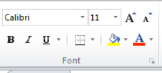
Figure 5–3. The Font button group

Many of the buttons here may look familiar to you if you've used Microsoft Word, and they do similar, though not identical, things here. Note the default Calibri 11-point font, the same one that starts you off in Word. Points are units of typographic measurement—units of height, to be exact—of which there are 72 per inch. Thus, 12-point text is one-sixth of an inch in height, for example.

Changing the Font

The basic principle behind making formatting changes is known as select-then-do; that is, you select a cell or cells (or even some of the text in a cell if that's what you want to change), and then execute the change. Thus, to change the fonts in a range of cells

1. Just select the range.
2. Click the down arrow beside the font field (where it currently says “Calibri” in Figure 5–3). This will present the Font drop-down menu, as shown in Figure 5–4.
   

   Figure 5–4. The Font drop-down menu

3. Just click the font you want, and you've made the change (you can reveal more fonts by clicking the arrows at the right side of the font window and scrolling down the font list).

Notice that Figure 5–4 shows a range that seems to contain nothing in it. It's true—the range is blank, but that's not a problem. That's because you can format a range prospectively, even before it contains any data. When you actually type the data, it will take on the changes you've brought about. Note also when you make a formatting change on a designated range, the range remains selected in case you want to make additional changes there.

Changing the Font Size

In much the same way, you can change the font size of the data. Just select your range and click the down arrow alongside the font size field (currently showing the default 11 points), and click the desired size.

Note, on the other hand, that the Font drop-down menu lists 11-, 12-, and 14-point sizes, but not 13. That's not a matter of superstition; rather, it's because Excel simply lists commonly used font sizes. If you really want your range to display 13- or 17-point-sized data, you can do the following:

1. Click in the font size field.
2. Type the size you want, as shown in Figure 5–5.
   

   Figure 5–5. Unlisted number: Entering a 17-point font

3. Then press Enter to finalize the change.

Now what about those two As stationed to the right of the font fields? They're called Increase Font Size and Decrease Font Size, respectively (see Figure 5–6).

Figure 5–6. A pair of quick ways to increase or decrease font size

Click the larger A on a range of cells, and the data there will receive a font size boost up to the next available interval in the font size window. That means that if the current size in a cell or cells is 12 points, clicking the large A will pump the size up to 14, which is the next higher size recorded in the drop-down menu. If you click the smaller A, those same 12-point cells with be downsized to 11 points, the next lower interval listed.

Using Bold, Italics, and Underline

Now let's turn to the B, I, and U buttons (see Figure 5–7).

Figure 5–7. B, I, and U (bold, italics, and underline)

These buttons represent bold, italics, and underline, respectively—and again, to format data with any or all of these effects, select the cells in question and just click the appropriate button(s). These three buttons behave as toggles, meaning that by clicking them in succession you turn their formatting effects on and off. Click the B button once, and the cells you've selected turn boldface; click it again, and the bold effect disappears.

Note, by the way, that the U button is accompanied by a drop-down arrow. Click it, and this little menu makes its way onscreen, as shown in Figure 5–8.

Figure 5–8. Between the (under)lines

Note the first of the two menu options is nothing but the default underline—what you'd normally get if you just clicked the U straight away. So why do you need it? Because if you click the Double Underline option, you'll indeed draw double underlines beneath data in the selected cells. Additionally, the Double Underline button will then appear in the Font button group, replacing the standard Underline, at least until you exit Excel completely or reuse the single underline (see Figure 5–9).

Figure 5–9. Seeing double

Determining a Cell's Formatting

You can learn a lot about the formatting of a particular cell by simply clicking in it and then scanning the information conveyed about it in the Font button group. So, if cell C12 is currently underlined and boldfaced, and features a Bauhaus 93, 12-point font, click C12 and you'll see this information in the Font button group, as shown in Figure 5–10.

Figure 5–10. What's happening in cell C12. The data there is boldfaced and underlined, and exhibits the Bauhaus 93 12-point font.

Notice that the B and U buttons are illuminated, telling us that those effects are activated in C12; and we're also told about the Bauhaus 93 12-point font.

Adding a Border

To the right of the U button you'll find the Borders button, which doesn't format cell data as such, but rather lets you inscribe lines around some or all the four borders of cells (see Figure 5–11).

Figure 5–11. Borderline call: The Borders drop-down menu

Again, the technique for drawing borders is the same as for other kinds of formatting:

1. Select the cells.
2. Click the Borders button, and select the border option of your choice from the drop-down menu.

Play around with these and you'll see how they work; particularly the All Borders and Outside Borders selections, which you may decide to use often.

All Borders draws borders around all the selected cells. This option can be particularly useful for emphasizing a particular group of cells (see Figure 5–12).

Figure 5–12. We've got you covered: The All Borders option surrounds all the selected cells' borders with lines.

Outside Borders limns a border around the perimeter of a range of cells, not individual cell borders. It's effective for singling out a range of cells for emphasis (see Figure 5–13.

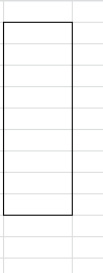
Figure 5–13. The Outside Borders option

You'll want to know about the No Border option, too, which removes borders around selected cells if you decide they're no longer needed:

1. Just select cells exhibiting the borders.
2. Click No Border, and the borders will vanish.

If you're wondering why you couldn't simply click the Undo button to achieve the same result, you could—maybe. Remember that Undo works in sequence, and if you decide you want to remove some cell borders well after you've drawn them, you'll have to undo all the commands you've executed in between, too.

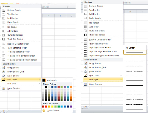
Figure 5–14. The Line Color and Line Style options

Adding Color to Your Cells

That leaves us with two remaining buttons in the Font button group: the Fill Color and Font Color buttons. Fill Color, as represented by the pail icon, has nothing to do with the fill handle discussed earlier; rather, it fills the selected cells with a color you choose from a drop-down menu (see Figure 5–15).

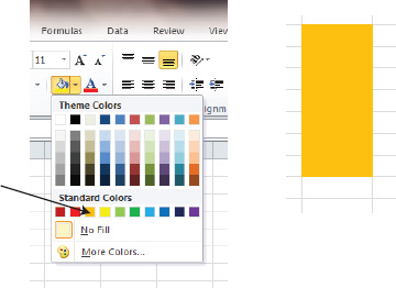
Figure 5–15. Click the arrow alongside the Fill button to produce this drop-down menu and result.

Use this option when you want to impart emphasis to selected cells. Note that the color you see right beneath the pail icon (the color underlining the pail) is the current fill default color—the color that will appear in the selected cells if you click the Fill Color button instead of its drop-down arrow. And if you want to turn off the current fill color tinting any cell(s), just select the cells in question and click the No Fill option.

The Font Color button, represented by the A, changes the color of the data in the selected cells. It too sports a drop-down menu exhibiting the same color options displayed in the Fill Color menu, as shown in Figure 5–16.

Figure 5–16. The Font Color drop-down menu. The Automatic option represents the default font color, black.

Just select your cells and click away.

Adding Extra Formatting

Finally, note that the Font button group has one of those dialog launcher arrows—that little indicator squirreled in the lower right of the group (see Figure 5–17).

Figure 5–17. There's that dialog box launcher again.

Click it and you'll bring up what's called the Format Cells dialog box (shown in Figure 5–18).

Figure 5–18. The Format Cells dialog box. Note the various tabs.

Note the various font-formatting options here, most of which you've already seen in button form in the button group. There are, however, a few additional possibilities here—namely in the Effects area, where you can draw a strikethrough line through data. Figure 5–19 shows an example.

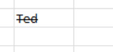
Figure 5–19. The strikethrough effect

Aligning (and Realigning) Your Data

The group to the immediate right of the Font button group is called the Alignment group. It's shown in Figure 5–20.

Figure 5–20. The Alignment button group

Its buttons don't quite change the appearance of data; rather, they reposition data in its respective cells. Recall that numeric data, or values, appear by default at the right edge of cells, while text data is positioned, or aligned, at the left. The Alignment buttons allow you to relocate the data to different positions, called orientations—both horizontal and even vertical—in cells.

Changing Horizontal Alignment

The trio of buttons in the lower left of the group (see Figure 5–21) controls the horizontal placement of data (you'll see these in Word, too).

Figure 5–21. The horizontal alignment buttons

What they do is pretty self-evident. Here's a quick exercise involving text alignment:

1. Click the far left button, Align Text Left, after you've selected a range of cells, and their contents will be shifted to the cells' left edges (of course, if you're working with text data, that's where they'll be anyway).
2. Click the next button along, called Center, and the data will zip to the center of its cells.
3. Click the third of the three, Align Text Right, to shunt the data to the right edge.

Thus, if you've entered values, the buttons will bring about the kinds of results shown in Figure 5–22.

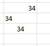
Figure 5–22. Right, left, and centered values

Keep in mind that many people like to center values down a column, enjoying the symmetrical effect that centered data brings. But you may want to think about that decision, because if your data contains values of different lengths you can wind up with something like what's shown in Figure 5–23.

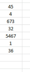
Figure 5–23. Out of whack: What centered values can look like

You see the problem—but it's your call.

Changing Vertical Alignment

The next set of buttons, Top, Middle, and BottomAlign do something more exotic (see Figure 5–24).

Figure 5–24. The vertical alignment buttons

They let you align data vertically, enabling you realize the kind of effect shown in Figure 5–25.

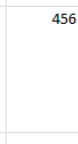
Figure 5–25. The sky's the limit with the Top Align button

Now, in order to make that happen, you need to learn how to heighten a row. We've already talked about widening a column; row heightening works in a similar way:

1. Move your mouse above the lower boundary of the row you want to heighten (see Figure 5–26).
   

   Figure 5–26. Placing the cursor here with let you heighten row 15.

2. Click and drag the boundary down until the row achieves the desired height. Release the mouse.
3. You can heighten multiple rows at the same time by dragging atop adjoining row headers (see Figure 5–27).
   

   Figure 5–27. Heightening several rows simultaneously

4. Then drag any one of the selected row boundaries to the desired height and release the mouse. All the rows will acquire the same new height.
5. Click anywhere to turn off the blue selection color.
6. If you've dragged too far you can also execute a row autofit by double-clicking a row's lower boundary.

Once you've completed that task, all you need to do is select your data and click one of the Vertical Align buttons to bring about the effect you want. Of course, Bottom Align is Excel's default—data will automatically position itself on the bottom of a row unless you decide to make a change.

Changing Data Orientation

The next alignment button, called Orientation, will let you do something even more unusual: incline data at an angle. Click its drop-down arrow, and you'll see the options shown in Figure 5–28.

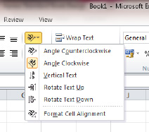
Figure 5–28. Everybody's got an angle: The Orientation drop-down menu

These options are pretty cool, but need to be used judiciously, as they reposition the data at severe angles. Select a cell and try the various orientations. You'll get some pretty striking results, which can work with both text and values. Just make sure that your audience will be happy to see a value that looks like Figure 5–29, for example.

Figure 5–29. That number—433—can still be used in formulas.

That's 433, and appearances to the contrary, that value is lodged in only one cell. All you need do to achieve this effect is select the cell(s), and select the Vertical Text option (shown previously in Figure 5–28).

The last drop-down option, Format Cell Alignment, will deliver you to the same Format Cells dialog box shown earlier—only this time the Alignment tab is pushed to the foreground, as shown in Figure 5–30.

Figure 5–30. Even more alignment options

Among other things, you'll see an Orientation area at its right edge. If you type in a number in its Degrees field, the data in cells you've selected cells will be pitched at just that angle (note the arrow in Figure 5–31). Also, if you click cells containing angled text and type 0 in the Degrees box, the data will be restored to its original, unangled appearance.

Figure 5–31. Select the cells you want to restore, type 0 degrees in the Degree field (you have to actively type 0 even if it's already displayed), and click OK.

Indenting Data

The next two buttons are titled Decrease Indent and Increase Indent, respectively, and all they do is push data in their cells slightly to the left or right by small increments, much in the way that the indent option works in Word. Each click advances or pulls back the data a bit more in their cells. Between you and me, I don't recall ever having used these buttons in an actual worksheet—but they're there (see Figure 5–32).

Figure 5–32. The Indent buttons

Wrapping Text

The next button, Wrap Text, is a good deal more useful. Clicking Wrap Text is the option of choice when you enter text in a cell that extends beyond its current column width and you don't want to widen the column. We've seen this problem before, of course, but Wrap Text proposes a different solution:

7. Enter the phrase shown in Figure 5–33 in cell B19.

Figure 5–33. Getting carried away: Too much text

8. Click back in cell B19 and click Wrap Text. You'll see what's shown in Figure 5–34.

Figure 5–34. Back where it all belongs

Wrap Text treats the current column width as a fixed margin and heightens the row instead, in order to confine the text within that margin. Wrap Text is thus an option you'll turn to if you need to maintain a column's width as it presently stands.

Adding a Title with Merge and Center

The final alignment option, Merge and Center, provides a set of suboptions in its drop-down menu, as shown in Figure 5–35.

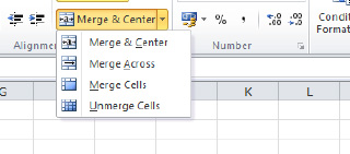
Figure 5–35. Merge and Center: Getting cells together

Merge and Center was devised to solve an old spreadsheet problem. Say you have a worksheet that currently looks like Figure 5–36.

Figure 5–36. Want that title to be centered among the month names? Stay tuned.

What if you want the Yearly Sales Totals title to be centered across the 12 months? Here's how to do it:

1. Say the month names you see in the screenshot span the range A2:L2 (remember, you can enter these names using the fill handle), and that the title Yearly Sales Totals appears in cell A1. Select cells A1:L1—that is, the range directly above all the months, in the row containing the phrase Yearly Sales Totals.
2. Now click the Merge and Center button directly (no need to activate the drop-down menu), and you'll see what's shown in Figure 5–37.

Figure 5–37. Middle ground: The title is precisely centered above the months.

Merge and Center does two things:

• It combines, or merges, all the selected cells into one megacell.
• It then centers the text across it.

This option spares you the challenge of figuring out exactly where to find the center point above the months.

You're far less likely to use the other two active merge options—Merge Across and Merge Cells.

• Merge Across lets you select a range consisting of several rows and columns, and turns each individual row into a single cell (see Figure 5–38).

Figure 5–38. Note the merge effect: Tuesday and July now each occupy a large, merged cell.

• Merge Cells lets you turn any range (which can include both rows and/or columns) into one supercell.

But as with Merge and Center, these only work properly when data is positioned in the leftmost cell of the selected range (these commands will work with completely empty ranges, however).

Finally, the awkwardly named Unmerge Cells option restores any merged cells back to their original state. Select the merged megacell, click Unmerge Cells, and all the original cells will reappear (see Figure 5–39).

Figure 5–39. Now Tuesday is back in its original cell, and all the cells that had been merged with it are back, too.

Inserting, Deleting, and Hiding Columns and Rows

Merging cells hints at some other important ways in which you can modify the structure of the worksheet itself, in addition to the data that the worksheet contains. There may be times when you need to insert or delete a row or column in the worksheet. Say you've constructed a list of employees along with identifying column headings, as in Figure 5–40.

Figure 5–40. The headings for an employee directory. Note the columns have been autofit.

It then occurs to you that you've inadvertently omitted a Salary field, which you want sandwiched between Telephone Number and Dept. You'll need to insert a column.

Inserting a Column or Row

As usual, there are several ways in which to do this. Here's one:

1. To insert a column, right-click anywhere on the column heading to the immediate right of where you want the new column to be inserted. In the example in Figure 5–41, you'd right click the E column heading, because you want Salary to be installed to the left of Dept.
   

   Figure 5–41. After right-clicking the E heading, click the Insert option.

2. Click Insert, and the new column will appear, as shown in Figure 5–42.
   

   Figure 5–42. Now you can type “Salary.”

   A different method allows you to insert a column by clicking anywhere in the column to the right of where you want the new one inserted:

3. Click a cell in the column to the right of where you want to insert the column.
4. Then click the Home tab, and choose Insert Insert Sheet Columns from the Cells button group, as in Figure 5–43.
   

   Figure 5–43. An alternative way to insert a column. Note the Insert Sheet Rows option, too.

   You'll get the same result—the new column.

   To insert rows, the procedures are nearly identical:

5. Here, the first method requires you to right-click anywhere in the row directly beneath where you want the new one to appear. Thus, if you want to insert a new row between rows 10 and 11, you right-click row 11, as in Figure 5–44.
6. Then just click Insert.
   

   Figure 5–44. Just click Insert, and the new row will appear above the current row.

To apply the second method to rows, do the following:

1. Click anywhere in the row directly beneath where you want the row to appear.
2. Click the Home tab, and click Insert Insert Sheet Rows from the Cells button group.

Inserting Multiple Columns or Rows

If you need to insert several columns or rows at the same time, you first need to select as many column or row headings as correspond to the number you want to insert. Thus, if you want to insert three columns, select the three column headings to the right of where you want the new ones to appear by simply dragging your mouse across the headings (not the worksheet cells), as in Figure 5–45.

Figure 5–45. Here, columns C through E have been selected; thus, the three new columns will appear to the right of column C.

You can then utilize either of the two insert methods just described (i.e., clicking Insert or Insert Sheet Columns). For rows, select multiple rows directly beneath where you want the new rows to appear.

What Inserting Does to Formulas

Inserting columns and rows may or may not impact existing formulas on the spreadsheet. If cell D12 contains

and you insert a column to the left of column D, the expression won't be rewritten. It will continue to read =AVERAGE(A12:C12), even though it now finds itself in cell E12. Excel tries to maintain the original formula relationships in the face of row and column movement. And that means that if you were to move all the values in cells A12:C12 to A5:C5 instead, you'd see

Again, that's because Excel assumes you still want to compute the average of those numbers, even though they've be moved.

Deleting Columns and Rows

The general approach to carrying out column or row deletions is, again, to select the columns or rows you want to delete using the selection techniques just described. Again, you can call upon either of the two insert methods, but this time of course you'll click Delete (see Figure 5–46).

Figure 5–46. Where to delete columns or rows. Note that in the second technique you'll click the Delete button alongside the Insert button.

Just keep in mind that if you're deleting cells whose data contributes to a formula, that formula will suddenly have nothing to work with—and instead of a result, you'll be left with an error message in the cell.

Hiding Rows and Columns

It's not unusual for Excel users to want to hide selected columns or rows—not so much in order to maintain the secrecy of the data, but to improve the appearance of a spreadsheet; perhaps columns with complex formulas don't need to be seen, or perhaps you'll want to hide those formulas so that you won't accidentally overwrite them; but if you do hide them, remember that all the data posted there remains active, and any cell references to them remain in force, too.

Again, there are two standard techniques for hiding. Here's the first:

3. Right-click the column or row heading you want to hide.

4. Click Hide in the resulting context menu (again, you can drag across multiple headings), as in Figure 5–47.

Figure 5–47. Where to hide columns or rows

Your worksheet will then exhibit a gap where the hide was executed, as shown in Figure 5–48.

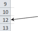
Figure 5–48. Row 11 isn't there, but its data is still usable.

The second technique for hiding columns and/or rows is as follows:

5. Select what you want to hide.

6. Click the Home tab, and then choose Format Hide & Unhide Hide Rows or Hide Columns from the Cells button group (see Figure 5–49).

Figure 5–49. An alternative way to hide columns or rows

Unhiding Columns and Rows

Unhide is one of those awkward Excel verbs, but that's the description for bringing back hidden columns or rows. Now, because the hidden areas can't be clicked directly—they're hidden, after all—you need to select columns or rows on either side of the hidden elements. Thus, if column K were hidden, you'd drag across headings J and L, as in Figure 5–50.

Figure 5–50. Trying to get back column K

Then right-click anywhere in that blue selection area and click Unhide (see Figure 5–51).

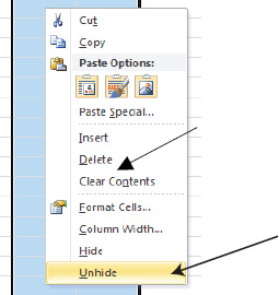
Figure 5–51. Just click Unhide, and K will reappear.

Alternatively, click the Home tab, and choose Format Hide & Unhide Unhide Rows or Unhide Columns from the Cells button group.

Inserting and Deleting Cells

You can also insert and delete selected cells, not just entire rows and columns—a possibility that isn't quite as obvious. If you click in cell A12 and carry out the Insert Cells command, for example, you'll push A12 down a row—but you won't push down row 12 in its entirety. Only the A column will be affected by the command. Any data in cell B12 will remain there, for example.

To insert or delete cells, select in the cell or cells with which you're working and either right-click the selected area and click Insert…, or click the Home tab and select the Insert Insert Cells… option from the Cells button group (see Figure 5–52).

Figure 5–52. Here, cells N8:N12 have been selected.

You'll see the dialog shown in Figure 5–53. If you click OK on the Shift cells down option, cells N8:N12 will be bumped down five rows—equal to the number of rows in N8 through N12. But no cells in other columns in the worksheet will be affected.

Figure 5–53. The Insert cells dialog box

To delete selected cells, select the cells you wish to delete and either right-click the selection and click Delete… or click Delete Cells… in the Cells button group (see Figure 5–54).

Figure 5–54. Where to begin deleting selected cells

Either way, you'll see the dialog shown in Figure 5–55. Just click the desired choice. Note that in the screenshot selection the cells' deletion would move the cells currently in O8:O12 one column to the left, so that they become N8:N12. You may have to think about this one—or better yet, experiment on a worksheet.

Figure5–55. The Delete cells dialog box

Formatting Values: Making the Numbers Look Good

Most of the work you'll do with Excel will likely be numbers-based, and many of the formatting options you need to know about impact numerical data only. Excel's Number button group (see Figure 5–56) contains a raft of ways to represent values that will make your data more meaningful.

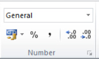
Figure 5–56. The Number button group

Turning Values into Currency

When you need to format numerical data so that it appears in currency form—dollars, pounds, euros, or just about any other denomination you can think of—just go to what's called the Accounting Number Format option, represented by the button shown in Figure 5–57.

Figure 5–57. Where to turn values into currency formats; note the dollar sign.

Just select the cells you want and click that button. The values should take on the currency format of your country (that country-specific setting should have been established by your computer's control panel before you purchased or when you first configured your PC), and exhibit these default characteristics:

• The indigenous currency symbol
• A comma for any value exceeding 999
• Two decimal points to signify cents, pence, or whatever the case may be

Click the Accounting Number Format button on cells containing the values 4523, 75, and 2, and you'll see what's shown in Figure 5–58.

Figure 5–58. Cashing in: Where to initiate the Accounting Number Format

Looking for additional currency symbols? Click the down arrow alongside the button and you'll see what's shown in Figure 5–59.

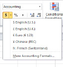
Figure 5–59. Currency exchange: Additional currency symbols

And here we need to issue a reminder. Substituting a $ for a £ in a value does not alter the numerical value of the data you've originally entered. In strictly mathematical terms, $4,523.00 is equal to £4,523.00; Excel won't calculate any currency exchange rates or anything of the sort. The currency symbol is just an embellishment of the number you wrote (as is the comma and the two decimal points). These are all format changes, and to repeat the declaration I issued at the outset of the chapter, formatting only changes the way a number looks.

If you need additional proof, do the following:

1. Enter 4523 in any cell.
2. Dress it up in a currency format.
3. Click back in the cell and direct your attention to the formula bar.

While your cell will display $4,523.00, the formula bar will reveal 4523.

And if you need still more symbols—if you're trading in Latvian lats or Bulgarian levs or any of a host of other international currencies, click the More Accounting Formats… option, shown previously, and you'll be brought to the dialog shown in Figure 5–60.

Figure 5–60. Scrolling for dollars … and other currencies

Scroll that ample list, and select your currency. Then click OK.

Figure 5–61. Symbolic gestures: Accounting and Currency formats

Working with Percentages

The next number button, Percent Style, is represented by—surprise—the percent symbol (see Figure 5–62).

Figure 5–62. The Percent Style button

Percent Style represents a number as a percentage, and as a result can be a bit tricky. Again, you just select the desired cell(s) and click the Percent Style button. Thus, the number 0.34 would appear as follows:

34%

That's easy enough, but keep in mind that the number 1 expressed in percentage terms is 100%, not 1%. If you're expecting that result, you'll have to enter .01 in the cell before you click Percent Style.

Punctuating Values

The Comma Style button actually does two things to the values you select:

• It adds a comma to any value exceeding 999.
• It posts two decimal points.

Thus, click the button on a cell containing 56802, and you'll get 56,802.00.

Formatting Decimal Points

The final two buttons on the lower tier of the Number button group are Increase Decimal and Decrease Decimal, important options that require a bit of introduction. As its name suggests, Increase Decimal adds a decimal point to a value with each click. In the case of a whole number, say 74, clicking Increase Decimal point results in

74.0

in which no real additional value is expressed. But if you had written the formula =4/7 instead, you'd originally see

0.571429

However, click Increase Decimal here, and you'll see

0.5714286

This adds a degree of additional precision to this repeating decimal.

On the other hand, if you narrow the column in which the preceding number appears, Excel will reduce its number of decimals so that you can continue to see the number. But it will also round the decimal off. Narrow the column here and you'll see

0.57143

Narrow it some more and you'll see

0.5714

and so on.

By the same token, type 4.67 in a cell followed by Decrease Decimal and you'll see

4.7

Click Decrease Decimal again and you'll see

5.0

But mathematically, that value is still really worth 4.67. Multiply it by 2 in a formula and the answer will come to 9.34, not 10. Again, we're only formatting the value, not changing its actual quantity.

Working with Dates: Dates Are Numbers Too

Enter the expression 3/4 in a cell and you may be in for a surprise. You know that 3/4 can't qualify as an actual fraction, because you've written it without the equal sign. So maybe it's just a bit of text, you may surmise. But it isn't; Excel will treat is as a date.

Depending on where in the world you live, that expression will be treated as either March 4 or April 3—but either way, it's a date. That's because Excel has decided that 3/4 and expressions like it will be regarded by default as a date, and assumes the date occurs during the current year—because people often like to write dates that way.

Treating 3/4 as a date is one instance of what's called Excel's general format, the default worksheet setting. The general format tries to understand what you have in mind when you enter data in a cell—before you've carried out any of the formatting changes discussed previously. Thus, Excel makes an educated guess about that 3/4, assigning it the status of a date unless and until you tell it otherwise.

But what you really need to know about dates is that they're numbers. In fact, March 4, 2011 is actually 40606—but what in the world does that mean? It means this: each date is assigned a sequenced number denoting the total days separating that date from January 1, 1900. Thus, March 4, 2011 arrived 40606 days after the baseline January 1, 1900—and that's a very good thing to know, because now you can determine the number of days between any two dates.

Here's an example:

1. Enter 3/4 in cell A2.
2. Then enter 1/15 in A3.
3. In cell A4, write =A2-A3, and you answer will be 48.

The 48 represents the number of days between January 15, 2011 and March 4, 2011, a result made possible because the later date has that numerical value of 40606, and the January date is really 40558. And 40606 – 40558 = 48.

Excel is well stocked with additional ways to format dates:

1. Click that January 15 entry in cell A3.
2. Then click what's called the Number Format drop-down menu (see Figure 5–63). This menu shows you what A3—which again is really 40193—would look like as per some of Excel's other formatting options.
3. Click the second Date option on the menu, and A3 will then display 1/15/11, replacing the current 1/15.
   

   Figure 5–63. The Number Format menu: Different guises for the same value

4. If you click the More Number Formats… options at the bottom of the menu, you'll be returned to the trusty Format Cells dialog box, this time with the Date option already selected (see Figure 5–64).
   

   Figure 5–64. Dates on the menu: Date options in the Format Cells dialog box

5. Choose whichever option you like, and then click OK. They're all different guises for the same number. And note that when you click any of the formatting possibilities, you'll see a preview of what the date is going to look like if you click OK, as in Figure 5–65.
   

   Figure 5–65. What you see is what you are going to get: Previewing a data format. The Sample area reveals the preview (see arrow).

Here's another tip: instead of directly entering 1/15 in a cell, you could have also entered 1-15. Excel's general format will also treat that expression as a date. And if you enter a date from the current year, you don't need to enter any reference to the year; 1/15 will be read as 1/15/11. But if you want to enter the same date from, say, two years ago, you'll need to enter 1/15/09.

Customizing Number Formats

If you're not quite happy with any of the formatting suggestions supplied by the Number Format drop-down menu, there are still more ways to remake the appearance of values.

The Special Formats Option

The Format Cells dialog box lists a Special option, which automatically formats values with four built-in looks that you can apply to values (see Figure 5–66).

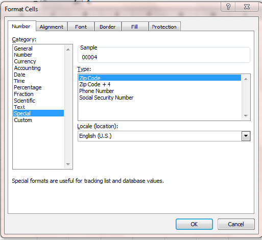
Figure 5–66. The Special formatting option

The Social Security Number option, for example, lets you type the nine-digit numbers without those pesky dashes that punctuate the numbers. Thus, if you select the desired cells and click Social Security Number, you'll be able to type 123456789, and have it automatically rewritten as 123-45–6789, sparing you the slightly odious task of remembering exactly where to enter those dashes.

Similarly, the Phone Number option will allow you to type 1234567 and immediately revise it to 123-4567.

The Custom Option

But there's still more. Excel's Custom option gives you the freedom to fine-tune numerical appearances precisely to your liking. While some Custom options are rather complex, there's one I use often that's quite simple.

You've probably noted by now that when you type a decimal value—say, .37—Excel ascribes this default format to it in its cell:

0.37

I don't know about you, but I don't like that leading zero; I want to see .37, and nothing more.

1. To achieve that appearance, select the cells you want to reformat and select Custom. You'll see the dialog shown in Figure 5–67.
   

   Figure 5–67. Decimal derring-do: About to excise that leading zero

2. Then click the 0.00 option, the third one down the Type list (see the arrow in Figure 5–68).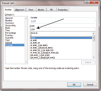
   

   Figure 5–68. Note that the Type field records the current format in the cell, with the leading zero in place.

3. Then click in the Type field and simply delete the leading zero. Note the Sample area shown in Figure 5–69.
   

   Figure 5–69. The zero has been zapped.

4. Click OK, and all decimal values in the selected cells will lose that zero.

Experimenting with the Custom options and observing how the content in the Sample area changes should prove instructive and useful.

Copying Formats (Not Data) with the Format Painter

Let's say you've formatted a cell with these characteristics:

• Using an Algerian 19-point font
• Colored red
• Italicized
• Festooned with an orange background

Something like Figure 5–70.

Figure 5–70. Have it your way: Your customized format

Hey—it's your worksheet. And you're so enamored with this collection of embellishments that you want to bring it to other cells. Of course, you could select those cells and then click the various options that gave rise to that thing of beauty in the preceding screenshot—but that's a lot of clicks. What you can do instead is copy and paste the format of that cell to other cells with the format painter. Here's how:

1. Select a source cell containing the formats you want to copy to other cells, as in Figure 5–71.
   

   Figure 5–71. The source and destination cells

2. Click the Format Painter button in the Clipboard button group (on the Home tab). The cursor will be accompanied by a paintbrush icon, as in Figure 5–72.
   

   Figure 5–72. Given the brush-off: The format painter cursor

3. Click and drag onto destination cells, as in Figure 5–73.
   

   Figure 5–73. Paint job: The format painter at work

4. Release the mouse. The destination cells should display the source formatting, as in Figure 5–74.
   

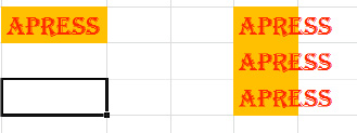
   Figure 5–74. The destination cells, after the source format has been copied to them. You might now want to widen their column.

The format painter copies only the formats characterizing the source cell, not the cell's data. It provides a handy way to export the formats into other cells, while leaving the destination-cell data intact.

Applying Ready-Made Formats with Styles

There may be times when you're having difficulty coming up with a nicely designed format that suits your data, and you may need something quickly—say, for a meeting or a presentation. Excel's Cells Styles option presents a large series of style options at the click of a mouse.

1. First select the cell(s) you want to restyle.
2. Click the Cell Styles drop-down arrow in the Styles button group, and you'll be presented with the dialog shown in Figure 5–75.
   

   Figure 5–75. Out of style? Choose one here.

3. Click any of these and see how your data looks (or just hover your mouse over the style option that interests you; the cell preview mode operates here, too).
4. If you reconsider your style selection, just summon that style gallery again and click another one (see Figure 5–76).

Figure 5–76. Just click a different style if you're not happy with the first one.

Customizing Your Own Style

You can also design your own styles. Let's say you want to turn that lovely Algerian, 19-point concoction into a style:

1. Format a cell as you wish. Here I've used
   • An Algerian 19-point font
   • The color red
   • Italics
   • An orange background
2. Select it.
3. Click the Cell Styles New Cell Style… option (in the lower left of the CellStyles dialog box). You'll see the dialog shown in Figure 5–77. Note that the cell's formatting attributes are recorded in the Style Includes area.
   

   Figure 5–77. DIY style

4. Type your own style name in the Style name field and click OK.
5. Click the Cell Styles button again and you'll see the dialog in Figure 5–78.
   

   Figure 5–78. My style, duly recorded

Not a catchy name, but you see the style listed under the Custom heading at the top of the dialog box. To delete a user-devised style, right-click its name and click Delete.

Applying Styles Quickly: Another Way to Access Formatting Options

As already stated, Excel isn't stingy about providing the user with various ways to do the same thing, and one way to carry out important formatting options uses the right mouse button click. Right-click a cell you want to format and you'll see what's shown in Figure 5–79.

Figure 5–79. The mini-toolbar, featuring formatting's greatest hits

Two objects suddenly appear:

• What's called the context menu, that tall column listing various command options, which by and large you can also access on the ribbon (e.g., Cut and Copy)
• The mini-toolbar, a collection of commonly applied formatting options gathered from various button groups. Just click the one you need (with the left button, by the way).

Note that the previewing feature described previously works here, too—rest your mouse over a formatting command before you click it, and the selected cells will show what the formatting change will look like.

Conditional Formatting

There may be times when you want to call special attention to certain cells. For example, you may be working with a list of test scores and want to quickly be able to tell which tests exceed a certain score, fall below that score, or both. Excel's conditional formatting feature lets you format cells so that they change their appearance only when they meet conditions you specify.

To continue with our example, with conditional formatting you can instruct any cell with a value greater than, say, 90 (a high test score) to turn blue—but only if it tops 90. Otherwise, the cell will continue to exhibit its original appearance. Thus, conditional formatting is an effective, and pretty easy, way to highlight certain cells scattered among a large mass of data (imagine reviewing 5,000 test scores!).

In fact, Excel gives the user many different ways to engineer conditional formats, some more complex than others. But many can be quite simple, even almost self-evident. Let's demonstrate one now, by turning to our test example.

1. Start by entering the test results from Figure 5–80 in cells C5:D15.
   

   Figure 5–80. Testing, testing … looking for scores above 90

   NOTE: Remember our objective: we want to be able to quickly identify all those scores that have achieved 90 or higher by having their cells turn blue.

2. Select the range of scores we want to conditionally format: D5:D15.
3. Click the Conditional Formatting button in the Styles button group on the Home tab (see Figure 5–81).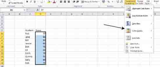
   

   Figure 5–81. The Conditional Formatting drop-down menu

4. Click the first option, Highlight Cells Rules. You'll see the conditional formatting rules shown in Figure 5–82.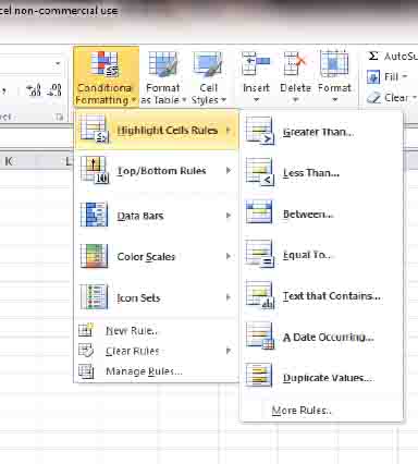
   

   Figure 5–82. Conditional formatting rules

5. Select Greater Than…, and you'll see the dialog in Figure 5–83.
   

   Figure 5–83. We're looking for cells greater than 90. The 80.5 is a default selection, which Excel computed by averaging the highest and lowest scores in the range.

6. Type 90 in the Format Cells that are GREATER THAN: field. We've established our condition: test scores above 90.
7. Click the drop-down arrow along the Light Red Fill with Dark Red Text entry. That's Excel's default, telling you that if any selected cell meets your condition, it will turn light red, and its text will appear as dark red. But we want our cells to turn blue instead, so click the Custom Format… option. You'll see the Format Cells dialog box, as shown in Figure 5–84.
8. Click the Fill tab, because we want the cells that meet our condition to turn blue, not the text in those cells.
9. Click a blue color in the resulting palette. Click OK.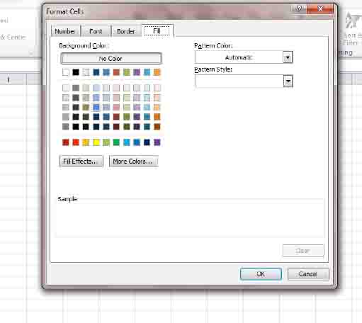
   

   Figure 5–84. Color scheme: Selecting a cell formatting color

10. You'll be brought back to the Greater Than dialog box. Click OK.
11. Turn off the blue selection color surrounding the test score range D6:D15. You'll see the content shown in Figure 5–85.
    

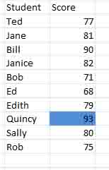
    Figure 5–85. Well done, Quincy!

To summarize, we used the conditional formatting feature to highlight all the cells that meet a condition we specified—in this case, all test scores over 90. We selected the cells we wanted to analyze, clicked the appropriate conditional formatting option (in this case the Greater Than… option), entered our greater-than-90 criterion, and then chose the color we wanted to apply to the cells that met the condition. And we see that only Quincy surpassed the 90 mark.

Looking for Scores Equal to or Greater Than 90

Now, what if we're looking instead for all scores equaling or bettering 90? There's more than one option here. We could click Highlight Cells Rules Between… instead of the original Greater Than…, which would reveal the dialog box shown in Figure 5–86.

Figure 5–86. One approach to looking for scores equal to or greater than 90

We'd then enter 90 in the first field, and 100 in the other, and then click OK. The rest of the process would be identical to the first exercise.

An Alternative Approach to the Same Result

The second option would take us to this command sequence:

1. Select Highlight Cells Rules More Rules…, as shown in Figure 5–87.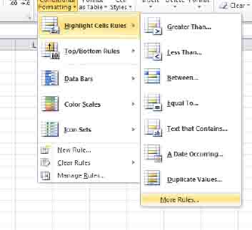
   

   Figure 5–87. Rules are made to be … followed.

2. Then select Format only cells that contain, and then greater than or equal to, as in Figure 5–88.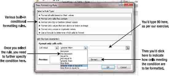
   

   Figure 5–88. Plan B

3. Click and then type 90 in the blank field to the right of greater than or equal to.
4. Then click Format and OK, and once again you'll be brought back to the Format Cells dialog box. And as with the other examples, you need to decide which sort of formatting change to introduce.

Just keep in mind that when you institute a conditional format, you can change the appearance of the text in cells (e.g., its font, color, or boldface/italics status) that meet your condition, as well as the color of the cell itself.

Some Additional Conditional Formatting Options

Again, Excel makes many other conditional formatting options available. Let's just look at two more.

1. Select the test data cells again and click Conditional Formatting Top/Bottom Rules. You'll see the options shown in Figure 5–89.
   

   Figure 5–89. Average white cells: Finding test scores above the class average

2. Click Above Average…, and you'll be brought to the dialog shown in Figure 5–90.
   

   Figure 5–90. Note that the above-average scores are tinted red in preview mode even before you click OK.

3. Click OK now, meaning that you're accepting Excel's Light Red Fill with Dark Red Text default conditional format. You'll see that all test scores exceeding the class average will exhibit exactly that—their cells will appear in light red, and the text in those cells will appear in dark red.

And conditional formats are dynamic, meaning that if you change the data with which you're working, the formats will change correspondingly. If you enter 100 for Edith's grade, for example, her cell will immediately turn light red with dark red text, because it now exceeds the class average—and Sally's grade of 80 will lose that formatting, because her grade will now fall below the average.

Turning Off Conditional Formatting

If you want to turn off your conditional formats and restore the cells to their original, black-text-on-white-background appearance, do the following:

1. Select the cells.
2. Click Conditional Formatting Clear Rules Clear Rules from Selected Cells (or from Entire Sheet, if that's what you want to do).

Using Data Bars: A Different Kind of Conditional Format

1. Here's one more conditional format option of a very different sort. Instead of coloring cells or their backgrounds on the basis of specified conditions, data bars occupy conditionally formatted cells with mini bar charts, which are proportioned to the values in those cells. Select the test data.
2. Click Conditional Formatting Data Bars.
3. Hover the mouse over the first Gradient Fill option, and you'll see the options shown in Figure 5–91.

Figure 5–91. Grades and gradients: Applying gradient bars to the test scores

What's happened—or what will happen if you go ahead and click—is the application of a mini–bar chart inside each cell displaying a test score. Note that the bar in Quincy's 93—the highest score in the class—fills the entire cell, and the other bars are sized in proportion to that 93. If you enter 100 in Edith's cell again, her bar that will occupy the entire cell, with the other cells proportioned to her grade.

Summary

Making your worksheets look good is an important part of the spreadsheet-building process. Excel's formatting options provide you with a heap of ways to do just that. Now we can move to another way—really, a group of ways—to present your data with striking visual appeal. The next chapter will introduce you to the world of charts.