Chapter 4

Number Crunching 101: Functions, Formulas, and Ranges

What makes Excel so powerful, and maybe even exciting, is its ability to bring something to the worksheet that wasn't there before. Taking a column of sales figures and finding their average or determining the highest score on a test—automatically—is really what Excel is about. If all you're doing is entering names and values on the worksheet without doing something to that information, you're probably using the wrong application—sort of a souped-up Word, only with cells instead of paragraphs. Learning how to compose your own Excel formulas and use Excel's built-in calculations, called functions, allow you to use some of Excel's real potential.

And you'll see that formulas tie into ranges—because your formulas often work with many cells at the same time (e.g., for computing sums, averages, and many other mathematical operations).

Of course, this is a mighty big subject, and learning all the things Excel can do in this area would require a book a whole lot larger—and more expensive—than you'd be prepared to pay for. What we're going to do here introduce the essentials—the things you have to know in order to get your money's worth—both from this book and from Excel.

Automatic Calculations with Functions

We'll start with functions and see how to carry out all sorts of calculations on your data.

Adding a Column of Numbers

So let's cut to the chase. Say you need to add that column of numbers—the classic Excel task.

1. In cells H3:H7, enter the values shown in Figure 4–1.
   

   Figure 4–1. It will all add up: The numbers we want to add.

   NOTE: Don't get the wrong idea—the actual values we've entered don't particularly matter, and more importantly the number of values populating in the column doesn't really matter either. The procedure for adding 50,000 values in a column works the same way as adding just 5.

2. Next, click in cell H8, click the Home tab, and choose AutoSum from the Editing button group (see Figure 4–2).
   

   Figure 4–2. The Editing button group

You should now see what's shown in Figure 4–3.

Figure 4–3. In summation: We're about to add all those numbers.

Let's take note of what we're looking at. Clicking the AutoSum button in H8 installs the expression shown in Figure 4–3. This expression uses Excel's built-in SUM function:

And what is that expression telling us? It's telling us that Excel plans to add all the values in the range H3:H7. Press Enter and you'll see the result, 267, in cell H8. Voila!

This expression is called a formula (you can tell a formula because it starts with an equal sign (=), and this formula displays the result of the SUM function. You can read the formula as “The contents of this cell equal the result of the SUM function.” In the “Customizing the Worksheet with Formulas” section later in this chapter, I will teach you how to write formulas from scratch. For now we are going to use the built-in functions, which make writing formulas quick and easy (and it's the functions that we really care about, because they do the hard work for us).

Now type 71 in cell H4, replacing the original 67. Cell H8 will now show 271. This demonstrates what's perhaps the single greatest contribution of spreadsheets to Western civilization: automatic recalculation. Once a formula has been placed on a worksheet, any change in the values used in the formula will immediately change the formula's result. There's no need to rewrite the formula—it delivers the new result automatically. Just change the contributing values, and the answer changes.

Returning to our example, we see that it works because SUM is programmed to add all the values in the cells directly above it (or to its left, if you're adding values in a row); that is, it adds the cells that actually contain a value. And that means that if we had encountered this range shown in Figure 4–4 in H3:H7 instead, and had clicked AutoSum again in H8, we'd have seen the result shown in Figure 4–5.

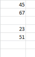
Figure 4–4. Something's missing: Adding (or trying to add) the values in this range

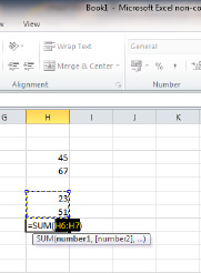
Figure 4–5. Same range, different result: Excel adds the cells containing values, until it encounters a cell that's either blank or contains text.

What Excel does here is incorporate each cell directly above H8 into its formula, until it lands upon a cell that's vacant—in this case, H5. Thus, Excel here would plan to add only the values in H6 and H7.

This is interesting, but it presents us with a problem—what do we do if we still want to add all the values in the range H3:H7?

Selecting the Range You Need

To remedy this, instead of pressing Enter as in the previous example—which produced the result 267—this time click and drag H3 through H7, as shown in Figure 4–6. Now the expression in H8 should read as follows =SUM(H3:H7), just as it did in our original case. Then press Enter.

Figure 4–6. Selecting the entire range you want

What you should learn from this second case—the case of the missing value in cell H5—is that the user can always override Excel's decision about which cells are going to be added with SUM. When you click AutoSum, Excel first displays the range it's about to add, as per the screenshots; and if you approve, just press Enter. But if you want to add the cells in a different range—which can be anywhere in the worksheet—not just in the same column—then click and drag across that range, and only then press Enter (see Figure 4–7).

Figure 4–7. Note that SUM is being calculated in a different column here, and that the range to be summed spans two columns.

Now here's another question: what does AutoSum do when you place it in a cell that's both at the bottom of a column and to the right of a row of data, as in Figure 4–8?

Figure 4–8. Placing the cursor at the bottom right of the data

In this case, AutoSum adds the values in the column, on the assumption that people more typically add values in the vertical direction.

Viewing and Editing Your Formula: Back to the Formula Bar

We've already talked about the formula bar—that long white strip bordering the upper rim of the worksheet, used for recording the contents of the cell in which you've clicked. Now you're going to see what the formula bar is really about. Click in cell H8 and direct your attention to the formula bar. You'll see what's shown in Figure 4–9.

Figure 4–9. Compare and contrast: Look at H8 and its contents in the formula bar.

Quite a contrast! The value 267—the result of the SUM we carried out—appears in H8, and of course that's what we want to see on the screen. But the formula bar displays the formula in H8 that gave rise to that 267. That's an important difference, because it lets you—or someone else—know that we didn't merely type the value 267 in cell H8; rather we performed a mathematical operation that brought about that total, and the formula bar verifies that claim. So if you really want to know what's going on in a cell, click in it and look to the formula bar.

And the formula bar provides an easy place in which you can edit the formula, too. For example, as in Figure 4–10, you can edit the range in the formula bar to add the cells in the range H3:I7 instead. Just click in the bar containing a formula, make the changes you need, and press Enter or click the Enter check mark alongside the formula bar.

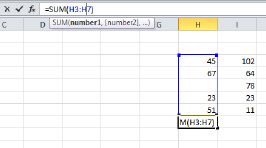
Figure 4–10. Editing the formula

In a nutshell, that's how to use AutoSum, a fast way to execute probably the most important mathematical operation you'll need to perform in a worksheet. But Excel has many more functions in its bag of tricks (including some additional ones that appear when you click the arrow alongside AutoSum), which calculate all sorts of things, most of which you probably won't need to know. It's not likely, for example, that you'll ever have to calculate the inverse matrix for a matrix stored in an array—whatever that might mean. But while you and I might not be concerned about that kind of capability, there are people out there who are, and there's probably a function in there that does just what they're looking for.

However, the more functions you know, the better, and there are at least a few that you should know about. If you click the drop-down arrow alongside AutoSum you'll see the list shown in Figure 4–11.

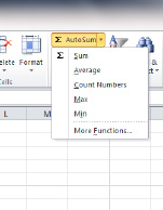
Figure 4–11. Additional popular functions

These work in an identical manner to AutoSum itself; that is, you can click in a cell directly beneath a range of values if you want Excel to automatically use that range, and then click any of the functions shown in the figure. Let's look at each one in turn. Table 4–1 summarizes them.

Table 4–1. Additional Functions You Can Access Directly by Clicking the AutoSum Button

Name	What It Does
Average	Calculates the average of a range of values; ignores cells containing text
Count Numbers	Counts the number of cells in a range containing values
Max	Calculates the highest value in a range of values
Min	Calculates the smallest value in range of values

Calculating an Average

So, let's see how to calculate an average, with the blank-cell rule from before in mind. Now, if you were to click Average, you'd get the AVERAGE function in cell H8, and you'd see what's shown in Figure 4–12.

Figure 4–12. Just your AVERAGE Excel function

Press Enter and you'll see 56.6 in cell H8.

And as with SUM, you can always drag your mouse across an alternative range if you don't like the one that Excel suggests. And there's no reason why you can't drag across several columns as well as down many rows. This expression is perfectly legal, then:

Displaying Values Based on a Certain Condition

Again, there are a couple of hundred other functions out there for you to explore, but we're going to illustrate just one more. It's called IF, and it carries out an action in a cell provided another cell meets a certain condition (or conditions) that you establish.

What does that mean? Consider this simple scenario: you're a teacher who's given an exam with a passing grade of 65. You want to be able to list your class scores on a worksheet and automatically determine at a glance which students have passed.

In cell I12, enter the grade 66. OK, we know the grade is a pass, but we could be assessing dozens, or even hundreds, of scores at the same time, where the pass/fail evidence in every student's case wouldn't be quite so clear, because you might miss a score as you visually scan a long column of scores.

Click in cell J12 and type =I. I know that's a rather cryptic thing to write, but we're stopping there because you'll notice that something is already happening on the screen, as shown in Figure 4–13.

Figure 4–13. What starts to happen when you begin to enter the IF function (or any function)

What's happening is that Excel already knows you've started to write a function. It knows because you've begun the expression by typing the = sign plus a letter (in this case I). This has triggered what's called the Formula AutoComplete, that drop-down menu that lists function names, narrowing down the selection as you continue to type letters. Since IF happens to be the first function starting with the letter I, the blue highlight you see in the screenshot lands on it. Then press Tab (not Enter), and you'll see what's shown in Figure 4–14.

Figure 4–14. The caption identifies the elements of the function.

The Formula AutoComplete is trying to tell you the kinds of things that make up the IF statement—things like logical tests. But for now we're going to just type. Inside that open parentheses type the following, and then press Enter:

You should see the word Pass in cell J12, as shown in Figure 4–15. We've done it. The student has passed the exam—and again, while we knew that already, we've let the cell make that decision, not us.

Figure 4–15. A passing grade—barely

Now type 60 in cell I12; the word Fail will now appear in cell J12.

Now I'll explain what we've written. The IF statement in its entirety reads as follows:

• I12>=65 is called a logical test, which is the condition that the value in cell I12 is asked to meet; that is, is the test score equal to or greater than 65? If it is, then what? Well, then the word Pass appears in cell J12—the cell in which we've placed this function.
• Pass—or "Pass", as it has been written, is called the value if true (see the caption in Figure 4–14), which is the result that will appear in J12 if the condition is met. Since in our first case, in which the student scored 66, the condition is indeed met, Pass appears in the cell.
• In our second try, in which the student scored 60, the word Fail appears instead. This is because the score hasn't met the condition (the logical test), and failure to meet that condition triggers the value if false (see Figure 4–14.—in this case, the word Fail.

Got all that? If not, with a bit of playing around with the expression (e.g., you could edit it to enter a different passing score), it will start making more sense. As usual, practice is the hidden ingredient.

Revisiting Function Structure

Now I'll offer a few general observations about how to use functions:

• You must write an equal sign (=) before you can use the function (functions can only appear in formulas).
• The equal sign is always followed by the function's name (e.g., SUM or AVERAGE).
• A parenthesis always comes next in the expression, and the function always concludes with a closed parenthesis, like so: =AVERAGE(A23:A72)
• The kind of information you enter between the parentheses varies, from ranges to logical tests.

Locating Functions in the Function Library

As already stated, Excel has hundreds of functions that do all kinds of things. When I was first exposed to functions sometime during the last century, I was mystified why anyone would actually want to use these curiously named things, and they seemed bewilderingly obscure. But as I began to learn more about spreadsheets, I began to appreciate the many uses to which functions can be put, and the more you know about them, the more you'll be able to do in Excel.

All of Excel's functions are stored in a collection of buttons in the Function Library button group on the Formulas tab, as shown in Figure 4–16.

Figure 4–16. Good reading: The Function Library

Table 4–2 briefly summarizes the types of functions contained in each group.

Table 4–2. Function Types

Group Name	Kind of Function
AutoSum	Contains the same function list you'll see when you click the AutoSum button on the Home tab.
Recently Used	Lists the last ten functions you've used.
Financial	Lets you perform many kinds of financial calculations, including interest projections and investment yields.
Logical	Includes IF and other functions that help you decide between alternatives (e.g., AND and OR). For example, the statement =IF(OR(A2>=65,A3>=65),"Pass","Fail") means that if either score in cell A2 or A3 equals 65 or higher, then the student passes.
Text	Contains functions that let you learn information about cells containing text. For example, =RIGHT(D12,2) will yield an answer of AB in a cell containing the text XYZ-AB, by identifying the two rightmost characters in the cell.
Date & Time	Lets you work with chronological data. For example, the function NOW(), which has nothing between its parentheses, will tell you the precise time when you enter new data in the spreadsheet, and will update whenever you enter new data.
Lookup & Reference	Lets you find particular data in a range, among other tasks. The VLOOKUP function, for example, can look up a person's income in a table and tell her how much tax she owes.
Math & Trig	Contains many mathematical and trigonometric functions, including SUM.
More Functions	Contains a host of additional functions, including ones that perform statistical and engineering tasks.

By clicking the arrow at the bottom of each button, you'll be able to view a list of all the functions assigned to that group; hovering your arrow over any name yields a brief description of what that function does. Figure 4–17 shows what you'll see if you rest your mouse over IF, stored in the Logical group.

Figure 4–17. Excel describes the function when you scroll over it.

If you go ahead and click IF, you'll be brought to a dialog box that prompts you to fill in the blanks—blanks consisting of precisely the parts of the function between the parentheses shown in Figure 4–18.

Figure 4–18. Look familiar? The dialog box prompts you to enter data in the three IF elements between the parentheses. In our test example, “Pass” is Value_if-True, and “Fail” is Value_if_False.

Thus, if you look back to that exercise, you would type I12>=65 in the Logical_test field, and and then supply the value_if_true and value_if false consequences, e.g., “Pass” or “Fail” (note that these between-the-parentheses elements are called arguments), and when they're all filled, you'd click OK. And as you click in each of the fields, a small explanation what the field does appears in the dialog box. If you click the Help on this function link in the lower left of the dialog box, you will be delivered a lengthier discussion of how the function works and is written. Just remember that each function will ask you to fill in a different set of blanks, depending on what it does.

Customizing the Worksheet with Formulas

While functions are an integral part of the spreadsheet process, there may be times when you need to do something more specific to your data, something that a built-in function can't anticipate. For example—what if you wanted to give every student a bonus of three points after a challenging exam? Or what if you needed to calculate the local sales tax on a series of purchases? Excel can't supply a function to carry out just those intentions, and so you may have to write a formula—or a series of formulas—which do the work you need done.

Formulas can be very simple, or can get very complicated. They can incorporate Excel functions, or they can exist in a stand-alone capacity. Here we're going to explore the essentials of formula writing, so you can get going and do real work with them.

Writing a Basic Formula

Formulas always begin with the equal sign. They follow with cell references, actual values, and one or more mathematical operators. OK—what does that all mean?

Let's see. Here's an example of a very simple formula:

And here's another one:

In the first case, we're adding 6 and 8—pretty obvious, but just remember to include that equal sign. Leave it out, and all you'll see in the cell is 6+8.

In the second case, we're dividing the contents of cell D3 by the contents of cell R9. Change the contents in either or both cells, and the result automatically recalculates, as usual. You can simply type that formula or click the respective cells—that is, type =, click cell D3, type the division sign (/), click cell R9, and press Enter (Figure 4–19):

Figure 4–19. Note that the two cells referenced by the formula are surrounded by borders as you write it.

Table 4–3 shows how Excel represents mathematical operators.

Table 4–3. Excel Operators

Operator	What It Does
+	Addition
-	Subtraction
/	Division
*	Multiplication
^	Exponentiation (4^2 means 4 squared, or 16)

And by the way, it's perfectly fine to combine functions with your own formula elements in the same expression; and as you grow more experienced, you'll probably be doing that sort of thing often. For example—you could write

This formula would add all the values in cells A12:A68, and divide that result by 7.

You could also write

This would divide 7 by the sum of all the values in cells A12:A68.

And that's just for starters. When you begin to see and appreciate how these various partscaninteract, you'll be making a leap in your Excel understanding.

Working Out the Order of Operations in a Formula

Once you start writing formulas, you need to keep something else in mind—something you may not have thought about since high school. Ask yourself, what result does this formula deliver?

Hmmm. You could be adding 32 and 4 and then dividing that result by 3, yielding 12—or are you starting with 32 and simply adding 4/3 to it?

That sort of ambiguity leads us to Excel's order of operations—a priority listing of which sort of mathematical operation is carried out first when a formula encounters the kind of mixed message just shown. Here's the listing, arrayed in order of priority (don't worry, I'll explain):

1. Parentheses
2. Exponentiation
3. Multiplication
4. Division
5. Addition/subtraction

Consider this formula:

Here, Excel takes the two values between the parentheses, 54 and 6, and adds them, yielding 60. It then multiplies that result by 3, and then subtracts 2 from 180, winding up with 178. Finally, 60 times 3 equals 180, and 180 minus 2 yields 178. The order of operations is confirmed:

1. Treat the values within parentheses as a unit.
2. Then give priority to multiplication, and then to subtraction.

What Excel won't do, then, is take the 60 and multiply it by 3 – 2, yielding 60. Play around with some of your own examples and the order of operations will become clearer.

Copying Formulas: More Than Just Duplication

I've already discussed how to copy data and formats through the format painter. But copying formulas introduces something new, something important. Let's see what that means.

1. Enter the test data shown in Figure 4–20 in a blank spreadsheet, starting at cell J7.
   

   Figure 4–20. Tough test

2. Save the file under the name Student Scores.
3. Now let's say that, because the scores are on the low side (these could be scores relative to a test score maximum of say, 120, but it doesn't much matter), the teacher decides to award a five-point bonus—and as a result, needs to write a formula that will impart that bonus to all the students. Enter the word Bonus to serve as a heading in cell L7, and in L8, write
   =K8+5

That little formula delivers a score of 82 to John, boosting his original 77. The question is how to award the same bonus to all the students, along with the implied question of what would happen if the class consisted of 100 students instead of just the five in our example.

The one thing the teacher won't do is write the formula for each student—that's way too inconvenient. The alternative is to copy the original formula down the L column, but we need to describe how that works.

There are several ways to copy a formula; we'll look at two of them. The first is very similar to the technique discussed in Chapter 2.

The Classic Copy-and-Paste Method

1. Click the cell you want to copy—in this case L8.
2. Click the Copy button via Home Clipboard Copy sequence.
3. Select the destination cells—in this case L9:L12.
4. Click the Paste button (in the Clipboard button group) or press Enter. You should see what's shown in Figure 4–21.
   

   Figure 4–21. Teacher with a heart: There's that five-point bonus.

Note that we obviously haven't copied John's grade to the other students—we've copied his formula; and when you copy a formula, Excel changes the cell references in the destination cells to reflect their distance from the source cell. That means that since our source formula reads

Bill's formula is going to read

because his data sits one row beneath John's. That one row down brings about a one-row change in his formula—from K8 to K9. And since Ed's grade-bonus formula is positioned in cell L12, it reads

to reflect its distance in rows—four rows, to be exact—from John's source formula.

This property of copied cell references—the fact that they record their degree of distance from the original source cell—is called relative cell addressing (or referencing), because the copied cells change their addresses relative to the source cell—the one that's being copied.

And that also means that if you were to copy a source formula horizontally (i.e., across a series of columns, not down a series of rows as per our example), relative cell addressing would change the column element of the cell address—its letter. Thus, if you copy =K8+5 one column to the right, the destination cell will read

Relative cell addressing is one of those Excel features you have to know, because copying formulas to destination cells is an extremely common part of the spreadsheet construction process. Relative cell addressing requires that you write just one formula in one cell—all you need to do next is copy that one formula to all the other cells with which you're working. Thus, if our hypothetical class consisted of 100—or even 1,000—students, you'd still need only construct one formula, which you'd then copy to all the other cells.

Next I'll discuss the second way in which to copy a formula. First, delete cells L9:L12, because we're trying out copy method number two. Then do the following:

1. Click back in the source cell, L8.
2. Click the fill handle—that small square holding down the lower-right corner of the cell pointer (see Figure 4–22).
   

   Figure 4–22. The fill handle revisited

3. Click the fill handle and drag it through cell L12.

Different technique, same result. And there's a cool, very useful variation on that technique you'll want to know about. If you click L8 and double-click the fill handle instead of dragging it, the source formula will be copied to all the cells through L12, too. This double-click method works when consecutive cells to the immediate left or right of the formula column have values in them. Thus, if K10 had been blank in our case, this technique would have copied the formula only through L9.

Moving Formulas: An Important Difference

You can move formulas with the techniques described in Chapter 2:

1. Select the formula-bearing cells you want to move.
2. Click the Cut command.
3. Click in the first destination cell.
4. Click Paste.

But when you're moving formulas, you're moving cell references, and here's where the difference lies. When you move a formula, the cell references in the formula don't change. That's because Excel assumes you want that formula to continue to refer to the same cells, even though it's being relocated.

Thus, if you write

in cell D2 and move it somewhere—anywhere—else, Excel will think that you still want the formula to add cells A2 and C2 (see Figure 4–23).

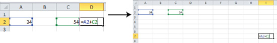
Figure 4–23. Moving the formula won't change its cell references. Notice it's fjrst been posted in cell D2, and in the second screenshot has been moved to I7 without an change in its cell references.

On the other hand, say you leave your formula in place in cell D2 but move the number in A2 instead, to cell B6. The formula will now state

That is, it will reflect the new destination of the values that contribute to a formula.

The bottom line is this: if you move a formula, or any of the cells that contribute to the formula instead, Excel assumes either way that you won't want to change the result of the formula—and so it makes the adjustments necessary to see to it that the result is unchanged by any changes in cell addresses.

Keeping a Cell Reference Constant with Absolute Addressing

As stated, understanding relative cell addressing is one of those must-know features that Excel depends on in order to, well, make it Excel. But there's an additional aspect to copying formulas that's just about as important.

Let's say our teacher isn't yet sure how large that grade bonus should be, and wants to try out different point awards to see how they affect the test grades. In cell N7, the teacher enters the number 4 instead, and rewrites the original formula in cell L8 to read

As you see, we've removed the number 5 and replaced it with a cell reference—cell N7, which currently contains the value 4. Thus, John's bonus score right now stands at 81, as shown in Figure 4–24.

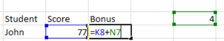
Figure 4–24. John's bonus-awarding formula

The advantage of using the cell reference is that if the teacher decides to change the grade bonus, all she needs to do is type that new bonus in cell N7 and John's grade will change automatically. The next step, then, is to copy this new formula to all the other students down the L column, as before, using any of the methods described previously. But this time something is going to go wrong.

When you go ahead with our formula copy, you'll see the content of Figure 4–25.

Figure 4–25. Not much of a bonus! Note the 4 points in cell N7.

What went wrong is that it appears that only John received the bonus. Why hasn't anyone else received it?

Absolute Addressing: When We Don't Want It to Work

Here's the answer. If you look at cell L9—the cell containing Bill's “bonus” grade (all you have to do is click L9 and look at the formula bar)—you'll see the following:

Well, that's supposed to happen, because of the relative cell addressing feature introduced previously. But what value is in cell N9? Nothing; cell N9 is blank. And 91 plus nothing is 91. Bill's score is unchanged.

And if you look at Dorothy's cell, L10, you'll see

Same problem. Both cell references have changed as we would expect, but again, there's nothing in cell N10—and so on for all the other students. Only John's bonus has kicked in. It's all because here we want all the students' formulas to refer to cell N8, the cell in which the bonus is stored. But because copied formulas exhibit relative cell addressing, they change their references relative to their distance from the source cell. What to do?

Introducing an Absolute Cell Address

What we do is edit the original source formula in cell L8—the cell containing John's bonus—to read

Note the obvious change: the addition of a dollar sign to the left of the 7, which identifies the row in the cell reference of N7. The dollar sign doesn't represent a currency format; rather, it freezes the 6 so that when you copy this formula down the L column, the cell reference N7 won't change.

To see what that means, delete the bonus data in the L column and enter

in John's bonus score cell of L8. Copy that formula down the column again. You should see the data shown in Figure 4–26.

Figure 4–26. That's more like it!

Save the workbook. At last, the bonus has been applied to all the students, because all the bonus cell formulas now reveal the N$7 reference, which won't change, even if you were to copy it down 1,000 rows. Check any bonus cell out to see what I mean.

And by the same token, if the test scores had been entered this way—that is, horizontally (with the data beginning in cell J9), you'd see the results shown in Figure 4–27.

Figure 4–27. The grades organized horizontally, starting at cell KJ9. Note John's formula in the formula bar.

John's bonus formula would now read

See why? Here, the dollar sign has been inserted to the left of the N, that part of the cell reference that indicates the cell's column letter. And we need to freeze the column letter here because John's formula has to be copied across a set of columns—and without the dollar sign, Bill's bonus formula would read

And there's nothing in cell O7.

In fact, you can freeze both parts of a cell reference (e.g., $N$7). Copying this reference in either direction—down a column or across a row—won't change the reference at all. This is good to know if you need to refer to that cell in a variety of locations in the worksheet.

It's true that newcomers to Excel sometimes find the subject of relative and absolute cell addressing a bit daunting at first, so don't be discouraged if you're feeling the same. Just bear in mind that you need that dollar sign only when formulas in different cells have to refer to the same cell over and over again—as with our last example, in which all the test scores need to refer to the same bonus-point cell—N7. Again, the advantage here is that if you need to change the bonus, you need only change the value in N7, rather than having to edit every student's formula. You could even recolor N7 to remind users that it's the only cell they need to change (recoloring will be discussed in Chapter 5).

Copying a Formula's Result Only

There may be times when you need to save a value on a worksheet that's been generated by a formula. For example—suppose you needed to record those student test scores with their bonuses to a different area of the worksheet for future reference. Well, that causes a bit of a problem—because the bonus-adjusted scores were brought about by a series of formulas. John's bonus-score cell (in the Student Scores workbook) doesn't really say 81—it says =K8+N7, and if we copy that expression to another cell, both the K8 and the N7 are going to change, due to relative cell addressing—and we won't see 81 in the destination cell as a result.

One way out of this problem is to copy the test scores as usual, but to paste them into destination cells using the Paste Values option, which pastes only the results of formulas, not the formulas the themselves. Let's try it out, and the concept will become clearer.

1. First, open the Student Scores workbook if you haven't done so already.
2. Then select and copy cells L8:L12, which contain the bonus grades.
3. Then click in cell P8, which will serve as the first of the destination cells to which we want to paste the scores (Figure 4–28).
   

   Figure 4–28. A different kind of copy and paste

4. Then, instead of clicking the standard Paste command in the Clipboard button group, click the down arrow beneath Paste. You'll see what's shown in Figure 4–29.
   

   Figure 4–29. Various paste options

5. Click Paste Values (the first button in the Paste Values group). The bonus test scores will appear in cells P8:P12 in addition to their original location—and they will appear as values, as if you had simply typed them There are no formulas in the destination range, and that means simply that the values in those cells won't be changed by data entry anywhere else in the workbook. They've been fixed.

   NOTE: Notice the two other Paste Values buttons in Figure 4–29. The middle button, Values and Number Formatting, will paste cell values plus any special formatting brought to those values (e.g., currency formatting). The right button, Values and Source Formatting, pastes the cell values along with any newformatting imparted to those cells (e.g., a different font or color). Again, we'll discuss formatting in Chapter 5.

Clarifying Cell References by Naming a Range

I've already introduced the pivotal concept of ranges, and you've already worked with quite a few of them besides. But there are a few additional aspects of ranges that are useful to know about.

For one thing, ranges can be named. That is, instead of working with a set of cell references such as C23:C42 and using that reference in a formula, you can substitute a name for it and use the name in the formula. For example, if this range contained test scores, you could name the range Scores—and instead of writing

you could write

Naming a range helps you and other people who view your worksheet to better understand exactly what sort of data has contributed to the range. Scores is a lot more revealing than C23:C42—and probably easier to write, too. And there are other advantages to naming a range, which we'll discuss here too.

Naming a range is easy, although as usual, Excel grants us several ways in which to carry out this task.

Naming a Range in the Name Box

The simplest technique is to name a range with the Name box:

1. Select the range you want to name.
2. Then click in the Name box—that field in the upper left of your worksheet—type your name, and press Enter. (see Figure 4–30)

Figure 4–30. Cells C23:C42, now named Scores

Try this with the preceding cells. It makes no difference whether the cells in a named range are empty or populated with data. Either way, you can name it. And if you click the drop-drown arrow to the right of the Name box, you'll see a list of all the range names you've added to the worksheet, as shown in Figure 4–31.

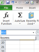
Figure 4–31. Where range names are listed—one of several places

Click any range name in that drop-down list, and Excel will select, or highlight, that range. It's a handy way to remind you exactly where a named range is located, and to navigate to it too.

Again, once a range is named you can apply it to a formula—and Excel helps you with that process, through the Formula AutoComplete feature discussed earlier. If, for example, you wanted to calculate the average of the Scores range, you'd do the following:

1. Begin by typing =AVERAGE (or really, =A, after which Formula AutoComplete will take you to functions starting with the letter A).
2. After you've gotten as far as =AVERAGE(, start to type the range name Scores. You'll see what's shown in Figure 4–32.
   

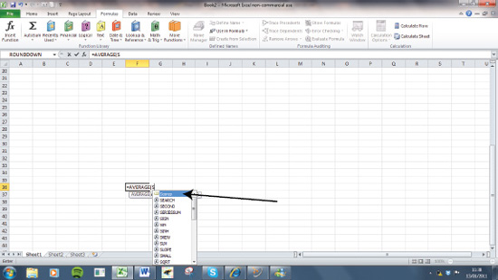
   Figure 4–32. Keeping scores: Note the Scores range listed.

3. Formula AutoComplete is at it again, this time supplying you with the name of a range, instead of its usual functions. Now press the Tab key to select Scores, type the closed parenthesis to complete the expression, and press Enter.

You can also define a range name with the Define Name option, available through the Formulas tab Defined Names button group Define Name. Click the button and you'll see the dialog in Figure 4–33.

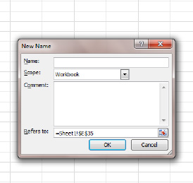
Figure 4–33. The New Name dialog box

Here you can type the range name, and even add a descriptive comment about the range if you like. The Refers to: field lets you type the range coordinates (e.g., C23:C42) without having to actually select those cells first, unlike the first technique.

Scope refers to the worksheets in the workbook in which you can use the range. By default, the scope of a range is defined as Workbook, and that means that you can use the range name in any of the worksheets that make up the book—so even if you've devised Scores on Sheet1, you'll be able to write the following in Sheet2 as well:

But if you confine the scope of Scores to Sheet1, you'll only be able to use Scores in formulas in Sheet1 (see Figure 4–34).

Figure 4–34. You can't get there from here: don't try using Score in Sheet2 now.

But why would you want to bother imposing such a restriction? Because you might be working with different sets of test scores on different worksheets, and you might want to use the range name Scores on each sheet—to represent only that sheet's scores. True, that's not a likely scenario, but Excel makes the option available.

Naming Ranges from the Data in Your Worksheet

Now let's look at yet a third way to construct range names, an approach that lets you derive the names from data you've already entered on the worksheet.

1. On a blank workbook, enter grades shown in Figure 4–35 in cells I9:L13.
   

   Figure 4–35. Title search: They're soon to become range names.

2. Save the workbook as Test Scores. Now select all the cells in that range and click Formulas Defined Names Create from Selection. You'll see what's shown in Figure 4–36.
   

   Figure 4–36. Range finder: Excel suggests range names culled from the titles in your data.

3. Click OK. Nothing will seem to have happened on the screen, but if you click the down arrow by the Name box, you'll see what's happened (see Figure 4–37).

Figure 4–37. Range names, batched up directly from the data—the titles in the left column and the top row

True to the Create Names from Selection dialog box, Excel has composed range names from the data in the left column and top row, by assuming that those areas are likely to contain header information that you could use as range names. That means that you can now write a formula like this:

Naming A Range Containing One Cell: Why Bother?

Now here's an important tip. You can assign a range name to exactly one cell—but why would you want to? Because when you copy a formula with a range name, that range is treated as an absolute reference—that is, the cells the range refers to don't change relative to their movement from the source cell that's being copied.

Thus, if we look back at our bonus-grade example, we could have named the bonus cell N7Bonus. Our original source formula in L8 (John's score) would then have read

And if we had then copied that expression down the column, all the other students' bonuses would have been correctly figured right away—without the need for those dollar signs. And that's because the range name Bonus would always mean N7—no matter where it's copied.

The Name Manager: Where They're All Ar-ranged

If your worksheet has many named ranges—and take it from me, it can—you'll find them all listed and inventoried in the Name Manager. You get there by clicking the Formulas tab, and choosing Name Manager from the Defined Names button group. Continuing with the preceding example, the Name Manager will look like Figure 4–38.

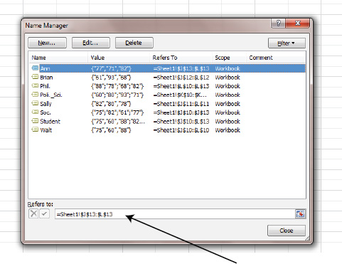
Figure 4–38. The Name Manger. Note the range coordinates indicated for the range Ann, which has been selected.

All the workbook range names are cataloged (along with names of any tables, which we haven't discussed yet; that's coming up in Chapter 7). You can edit the cell coordinates of any range by clicking its name in the list and typing new cell references in the Refers to: area. And by clicking the Edit… button, you'll be brought to a dialog box in which you can change the name of an existing range (see Figure 4–39).

Figure 4–39. Misspelled it? Call the range Anne instead.

And by clicking the New… button you'll be brought to the same New Name dialog box shown earlier when you clicked the Define Name button—so that's still one more way to initiate a new range name.

There's one more feature of the Name Manager you may want to know about: its ability to let you delete range names. Click the Delete button (or press the Delete key on your keyboard) on any range name in the list and you'll spark a prompt that asks if you're sure you want to go ahead. Click OK and the name will disappear. But don't worry—the data in the range remainsin its cells—you've only deleted the range name.

Summary

Call it number crunching or whatever you please—but however you characterize it, knowing how to write formulas and deploy Excel functions takes you to the heart of the spreadsheet enterprise. The more you know about Excel's capabilities, the more you'll be able to do with your spreadsheets, and while acquiring that knowledge takes a bit of practice, the investment should pay off. Once you get the hang of it, you'll come to realize there isn't much you can't do with Excel.

Next you'll see how to make all those numbers look good by learning about Excel's many formatting features. Just turn the page, and you'll see how to give your data a makeover.