Chapter 2

Getting Around the Worksheet and Data Entry

The Journey Starts Here

Whether you use a map, a satnav, a web-drawn itinerary, or do the retro thing instead and question an actual human being, any trip begins with knowing where you're going, knowing how to get there, and then deciding what to do once you've pulled into your destination. Your travels across an Excel worksheet aren't much different. You need to know where you want to go and how to track that destination down; and once you're there, you need to know how to fill that destination with the data that'll make the worksheet do what you want it to. It's a work sheet after all, and we're going to start doing that essential work now.

Looking Around

The grid in Excel is a good deal larger than what you're viewing on screen, and that's putting it mildly. In fact, every Excel 2010 worksheet contains 1,048,576 rows, probably way more than you'll ever need, and probably more than your computer could handle anyway were all those rows to be filled with data. And each workbook is outfitted with 16,384 columns, raising an obvious address question: if the 26^th column is called Z, then what does Excel call number 27? The answer: AA, followed by AB, etc. And when Excel runs out of double-letter combinations—at column ZZ, it adds a third letter, yielding AAA, and so on—all the way down to column XFD. Thus, ABC123 is a perfectly legal cell address.

Getting Around a Worksheet

Now in order to enter data in any cell you have get there first, by maneuvering the cell pointer into the desired address. Excel gives you many ways of getting there. Here are some of the standard ways:

You can utilize these navigational techniques with the keyboard:

• The Enter key—pressing Enter moves the pointer down one row.
• The Arrow keys—pressing any of these moves the pointer in the appropriate direction. That means the down arrow really does the same thing as Enter when you're navigating to the next cell– it takes you down one row.
• Tab—moves the pointer one column to the right.
• Shift-Tab—moves the pointer one column to the left. (But the Backspace key won't work here!)
• PgDn/PgUp—when pressed moves the pointer down or up one screen's worth of rows. Keep in mind that because you can change the height of rows, the number of rows you travel with these command may vary.
• Alt-PgDn/Alt-PgUp—A less-well-known pair of keyboard combinations. Pressing Alt-PgDn advances the pointer ahead one screen's worth of columns. Pressing Alt-PgUp takes the pointer back one screen's worth of columns. Again, because you can modify the width of columns, the distance you'll travel could vary.
• Ctrl-Home—a surprisingly useful combination. Ctrl-Home takes you to cell A1—the first cell in the worksheet. It's good to know about when you've travelled a long way across the worksheet, and you need to get back to the sheet's beginning.

Consider this scenario, then: You're in cell B22 and you want to make your way to cell Z18. You can click the right scroll button until the Z column appears on screen. Then just click on Z18 (the column letter doesn't have to be upper case, by the way). Try it! Of course you can get to your cell destination with the mouse, by simply clicking it onto the cell to which you want to go (note that unless otherwise indicated, all mouse clicks call upon the left button).

You can also use the Name Box to visit a cell. Just click into the box, type your cell destination, and press Enter. Voila—you're there.

Figure 2–1. Note the cell pointer in cell B7. Typing H1 in the Name box in pressing Enter takes you to….cell H1.

The Name Box is a cool way to travel long distances in the worksheet with precision -so if you need to get to cell XY38451, and fast, just type it in the Name Box and press Enter. Now want to get back where you came? Press Ctrl-Home, and you're returned to cell A1.

This table summarizes the techniques we've described:

Table 2–1. Navigational techniques summarized

Technique	Type of Movement
Enter key	Moves one row down
Shift-Enter	Moves one cell up
Tab	Moves one cell to the right
Shift-Tab	Moves one cell to the left
Arrow keys	Moves one cell in desired direction
Page-Down/Up	Moves one screen's worth of rows up or down
Alt-Page Down/Up	Moves one screen's worth of columns right or left
Ctrl-Home	Always moves to cell A1
Name Box	Moves to cell whose address you've typed in box after
Mouse	Enables user to click into any cell
Scroll buttons/bars	Moves to a new area of the worksheet; but does not directly select any cell

Remember that when you travel to any cell the current location of the cell pointer is always recorded in the Name Box.

Selecting Multiple Cells

In the course of your spreadsheet activity you may decide that you need to highlight, or select, more than one cell at a time. Why? There are several reasons you may want to do this, including these:

• You want to format the data in a group of cells all at the same time. For example: You want a group of numbers—perhaps a very large group—to display that currency format we spoke about earlier. By selecting all those cells simultaneously you can introduce the currency format to all of them, rather than having to change each cell individually. (See Chapter 4.)
• You may want to copy, or move, or delete, a group of cells at the same time. (See later this chapter.)
• You may want to print some, but not all the cells, in a worksheet. To carry this out, you'd first need to select just the cells you want to print. (See Chapter 8.)
• You may want to subject a group of cells to a mathematical operation- say, add the numbers in certain cells. (See Chapter 3.)

Selecting multiple cells, then, is your way of informing Excel exactly which cells you want to modify or work with.

There are several related ways in which you can select cells, and they're all pretty easy. The standard way is simply to click in the first cell you want to select, hold down the left button, and drag with your mouse across, or down, the other cells. The technique is very similar to the way you'd select a group of words in Word.

Thus if I wanted to select cells A6 through A19 I'd

1. Click cell A6.
2. Hold the left mouse button down.
3. Drag to cell A19.
4. Release the mouse.

Carry out this sequence, and again, your screen should look like this:

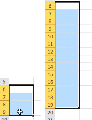
Figure 2–2. Selecting cells. Start by dragging (left screenshot) and when you've selected them all, release the mouse (right screenshot).

Note that the cell pointer—the thick black border—has expanded to include all the selected cells, which have turned temporarily blue (with the exception of A6, the first cell we've selected.(WhyA6 hasn't changed color will be discussed a bit later in more detail, but the blank cell represents the cell in which the data will go when you start to type. It's the blue color that tells you that these are the cells you've selected. Now you can go ahead and reformat the cells, or copy or print them (of course you'd want to put data in them first!)

Now of course you're eventually going to have to turn off the selection area in order to go ahead and do something else. To stop the selection process and banish the blue from your screen, just click your mouse, or press any arrow key.

Selecting Cells Down and Across the Worksheet

And when we select cells, we're not restricted to cells in one column. Once we've started to select we can keep that left mouse button down and drag to the right (or left, if we have room in that direction, or even up) as well, and select cells in additional columns:

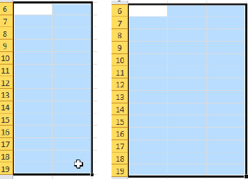
Figure 2–3. Selecting rows and columns, as we start to drag to the right

Selecting Cells with the Keyboard

You can also select cells with the keyboard. Click in the first cell you want to select, release the mouse, and then

1. Hold down the Shift key.
2. Leaving the Shift key down, tap any of the arrow keys in the direction of the cells you want to select.
3. You can change arrow keys as you proceed, so that you can select cells to the right of the start cell by tapping the right arrow key, and then begin to select cells downward by tapping the down arrow key.

Selecting All the Cells

Now back to that Select All button:

Figure 2–4. Remember—it's to the left of the A column heading, and above row heading 1.

Remember that clicking Select All highlights all the worksheet cells at the same time—all 1.7 billion or so of them. You'd turn to Select All, then, if you wanted reformat all those cells uniformly—say to implement the same font change in all of them. (Note: clicking Ctrl-A will also normally select all worksheet cells. (There's an exception to this rule, though: if you click anywhere in a group of consecutive cells that contain data—called a range, a topic which is coming next—Ctrl-A will select only those cells.)

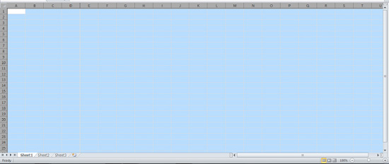
Figure 2–5. Complete coverage: what the worksheet looks like when you've selected all its cells

As we just indicated, a group of adjoining cells of the kind we've illustrated above is called a range, a key spreadsheet concept. Knowing how to identify ranges in formulas—something we're going to learn about soon—will enable you to work with large numbers of cells at the same time: to add the numbers entered in those cells, calculate their average, find the smallest number among them, and to carry out a nearly unlimited number of other tasks.

Still One More Selection Technique—The Name Box

And while we're at it, here's another cool way to select a range. You can click in the Name Box and type a range reference, something like

Figure 2–6. Entering range coordinates in the Name Box

Now what does that mean? It means we want to select all the cells from A12 though C23 (including A12 and C23). That's what the colon does—and if you press Enter next, all those cells will be selected.

Entering Text and Data

Data entry in Excel is as easy as it is important. Just select the cell you need, and type the entry—although that doesn't quite finish the process. When you type in Word, all you do, after all, is…type. But data entry in Excel requires an additional, but simple step. You need to confirm what you've entered with an additional command—almost always a navigational keystroke or mouse click.

Let's illustrate. The typical way to enter data is to select a cell, type whatever you want, and press the Enter key—and that's it.

Figure 2–7. Note the cursor alongside the letter l in the first shot. That indicates that you're still “in” the cell. When you press Enter, the cell pointer travels down one row.

Pressing Enter does two things:

1. It ”installs” whatever you've typed in the cell
2. It bumps the cell pointer down one row, as Enter normally does—nothing new there (as you'll see, there's an exception to this rule—when you select a range and then enter data into its cells).

That's the way it works—type your data in the cell, and press Enter—OR an arrow key, OR PgDn or PgUp, OR click the mouse into another cell. Typing data into a cell and following it up with say, a tap of the right arrow key, also does two things: it installs the data, and then in this case delivers the cell pointer one column to the right. Completing the data entry with a mouse click instead will simply land the cell pointer into the cell in which you've clicked—after the data has been installed in the original cell. I told you it was easy. The idea is that the pointer moves in the desired direction after carrying out the data entry.

There's also another way to carry out the data entry process. Select your cell, type away, and instead of executing one of the standard navigational moves we've described above click the gray check mark alongside the formula bar:

Figure 2–8. Getting ticked off: Completing the data entry process by clicking the gray tick

This click-the-tick approach will also finish off the data entry as with all the other techniques, but this time—and unlike the other methods listed above- will leave the cell pointer in the same cell. Note also the X to the left of the tick; click it instead and the 445 you've started to type above will be canceled

Aligning Your Data—Where It Appears in the Cell

Now let's look at a little more closely at the data you'll enter and how they appear in cells. When you type a textual entry the results appear left-aligned—that is, starting at a cell's left edge—by default, and that's simply because our Roman alphabet proceeds from left to right. But type a number—or what Excel calls a value, and it will position itself by default—that is, for starters—at the cell's right edge, because our number system is Arabic, extending right to left:

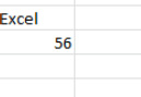
Figure 2–9. Choosing sides: Text aligned left, numbers right

Text data entry differs in some important ways from its numeric cousin. For one thing, if you type a lengthy phrase in a cell—and you can actually type over 32,000 characters in a cell—Excel will allow the excess text to spill into adjoining columns:

Figure 2–10. Crossing the line: a text phrase advancing into other cells

Just type away and let the text do its thing, bearing in mind that, appearances to the contrary, all the text you see in the above screen shot inhabits just one cell—the cell in which you started to type. That's all perfectly legal. But crossing cell boundaries can cause a problem.

Let's say the text we see above has been inscribed in cell B6. If we go ahead and type an entry in cell C6—the cell to its immediate right, we see something like this:

Figure 2–11. Now you see it, now you don't: The case of the missing text.

What happened? What happened is that the new phrase in C6 is simply claiming its own turf, so to speak. C6 was empty, after all, and all we did was enter a bit of text there—obscuring, but notdeleting, that part of the text in B6 that had overstepped its bound.

And how do I know that none of the text in B6 has been deleted? I can verify that fact by clicking on B6 and looking at the Formula Bar. You'll see

Figure 2–12. All there: the text in B6, revealed in the Formula Bar

Now we can begin to understand how the Formula Bar reveals the data you've entered in a cell. By that I meant that a glance at the actual cell doesn't always tell you what's really going on inside of it, and we'll see more evidence of this when we starting looking at formulas. Here we see that because of the data in C6, some of the phrase in B6 isn't visible—at least not on the worksheet itself. And if you were to go ahead and print the worksheet in its current state, the text in B6 would remain eclipsed as you see it above. But the Formula Bar reassures us that that it's all still there just the same.

Widening and Narrowing Columns

But that explanation still leaves us with the problem: we can't see the whole phrase in B6—and we want to. It's a classic spreadsheet dilemma—and the way to resolve it is to widen the column containing the “missing” text, revealing it completely on the worksheet.

There are several ways in which to widen Excel columns, and we'll explore what are probably the two most popular:

• Altering a column manually
• Using the auto-fit feature

Altering a column manually

Let's try the first method to widen a column:

1. Position the mouse over the right border of the column you want to widen—in this case column B—and click (don't release the mouse). You'll see:
   

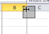
   Figure 2–13. The first step toward widening a column. Note the double-arrowed cursor.

2. Now drag the column boundary toward the right. You'll see the B column expand, revealing more of the text in B6 as you drag. When you've exposed all of the text, release the mouse.

That was easy, wasn't it? Just click on the right column boundary (it must be the right), and drag to widen. Just keep in mind that you need to click on the column boundary, and not on row 1 of the worksheet in order to carry out this task.

If you want you can narrow a column, too, by dragging to the left, in the same way.

Now that's pretty neat, but the process is slightly hit-or-miss and trial-and-error—because if you‘ve written a very lengthy text phrase in a cell, you may have to try the click-and-drag repeatedly until you‘ve widened the column to precisely the dimension you want. And that takes us to Method 2—the auto-fit.

Using the Auto-fit Feature

Let's try an auto-fit:

1. As with the Method 1, glide the mouse atop the right column boundary, until you see the double-arrowed cursor.
2. Double-click the mouse. The column should be widened to reveal all of the contents of the cell.

   Got that? Again, it's called auto-fit, and we see that double-clicking any column's right boundary resizes the column until all the data in that column is revealed. And that also means that if you've entered data into many cells in the B column and many of them exhibit obscured text, a double-click will widen the column to reveal them all. In other words, the auto-fit resizes the column to the width of the widest data entry in the column.

   You can execute an auto-fit on several columns at the same time. That means that if several columns suffer from the obscured-text-syndrome at the same time, you can widen them all in one shot. Here's how: Let's say that columns A through D all have data in some of their cells which are hidden by data in the adjoining columns, something like this:

   

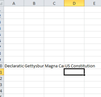
   Figure 2–14. But the words get in the way…four columns' worth of obscured text.

3. Click atop the first column heading you want to auto-fit (in this case, A)—and not its boundary, this time—keep the left button down, and drag across the headings of the adjoining columns you want to auto-fit:
   

   Figure 2–15. Selecting the columns by their headings

4. Double-click any one of the column boundaries selected—and all the columns will be auto fit:
   

   Figure 2–16. Fit to be tried!

5. Then click anywhere on the worksheet to turn off the blue selection color.

Pretty handy. Just remember that this multi-column auto-fit won't engineer identical widths for each column, because each width is tied to the widest entry in each column.

Entering Numerical Data—How it's Different

Now let's say a few words about entering values—that is, numbers. The basic techniques are identical for text entry: select a cell, type the value, and conclude the process with a navigational keystroke, mouse click, or that green tick. And don't worry about commas, decimal points, and currency symbols. Those are formatting embellishments that don't change the actual value you've entered.

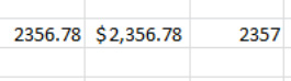
Figure 2–17. Some ways in which you can format values. Note the rounded off value in the third case.

So far so good. But there's a quirk about values you'll want to know about early on: Excel won't allow a large value to barge across into the neighboring column. That is, if you type 1000000000—however that value is translated into English—Excel simply will prevent it from trespassing into the column next door. So what does Excel do instead?

It does one of several things, depending on what's gone on in the worksheet before you entered the value.

By default, Excel carries out a kid of automatic auto fit on a lengthy value—that is, it will automatically expand the column to display the value in its entirety, without you having to double-click the column boundary.

But if you had already narrowed that column before you entered the value, Excel assumes you had a good reason for having done so, and leaves the column width alone. So instead, it does one of two things:

Displays the value in scientific notation, so it looks something like Figure 2–18. While you probably haven't seen a value expressed that way since high school, it does represent a more compact way of displaying the value in a narrowed column.

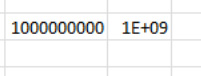
Figure 2–18. Remember these? A long value in scientific notation. The two values are identical.

But if the column is very narrow, such that it can't even accommodate the scientific notation, Excel displays the data as shown in Figure 2–19. Called pound signs in the US and hash marks in the UK, they tell the user that the column is simply too narrow to display anything else. Pound signs don't suggest you've made a mistake—what they always mean, rather, is that a value's in there (never text), and you just can't see it. All you need to do here is to widen the column—but truth to be told, you can leave it as is, if you want to only use it in formulas and the like.

Figure 2–19. There's a value in there somewhere, and it's the same as the one you can see.

Entering Data into a Selected Range

Now let's get back to a data entry issue I pointed to earlier, but didn't discuss. You'll recall that when you select a range of cells, the first cell in the group remains white—that is, it doesn't turn blue:

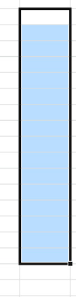
Figure 2–20. Drawing a blank: the first cell in the selected range won't change color.

Time to explain why. The first cell in a selected range maintains its original white appearance to let you know that when you start typing, the data will enter that cell. Moreover, if you conclude that data entry by pressing the Enter key, the range remains selected—and the next cell turns white:

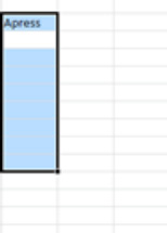
Figure 2–21. Type now and the data will once again enter the white cell.

You get the idea. Each tap of the Enter key turns the next cell white, designating the cell into which you'll be entering data.

But you may have a question about this sequence of events, because we don't appear to be learning anything new here. After all, pressing Enter always takes you down one row—so what's really different here? Good question.

The answer can be gleaned by considering this range selection, in this case L9:M18 (just to get you accustomed to range references):

Figure 2–22. A two-columned range selection

Here's the point. If you enter data in each cell and press Enter, you'll once again bump down the column, for example:

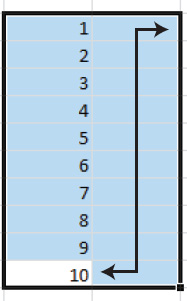
Figure 2–23. Right now you're in cell L18.

Now if you type a number and press Enter, you won't descend down a row; rather, you'll shoot up to cell M18—the first cell in the second selected column:

Figure 2–24. Staying in range

That's what it's about. Press the Enter key after you enter each item in a selected range and the white cell stays within the range bounds, rather than simply plunging down the column as it normally does. And again, after you've entered all the data in the range, click anywhere onscreen; the blue disappears, and the range is de-selected.

Using Auto Fill to Speed Up Data Entry

By now you may have taken notice of the small rectangle holding down the lower right corner of the cell pointer. It's called the fill handle:

Figure 2–25. There it is.

Why is the fill handle so named? It's because, among other things, you can fill a range with a collection of sequenced data—but what does that mean?

Copying a Value with Auto Fill

First, if you enter just one value or text item in a cell and drag on that cell's fill handle, you'll copy that item to as many cells as you drag. Thus if I enter 2 in a cell, click back into that cell and drag on the fill handle down its column, I'll copy the 2 into as many cells as I want:

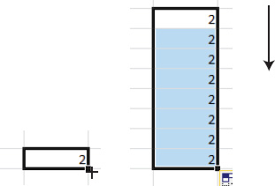
Figure 2–26. One way to use the fill handle: to copy a value

Auto Filling a Numeric Sequence

To see what I mean:

1. Type the values 1 and 2 anywhere in a column in adjacent rows.
2. Then select those two cells and release your mouse—an important step in an auto fill, which is what we're about to do:
   

   Figure 2–27. Having your fill—selecting the cells

3. Then glide the mouse directly over the fill handle. You'll see a slender black cross:
   

   Figure 2–28. A new kind of cursor

4. When you see it, click on it, and drag it down the column for as many rows as you wish. You should see:
   

   Figure 2–29. Value-added: auto fill at work

Pretty cool, no? What we did is start with just two values, which established a fill interval—in this case an interval of 1 (the 2 minus the 1). That tells Excel that every subsequent value will receive an increment of…1.

But you can really stipulate any increment you want. Start by entering say, the values 2 and 5 instead, and you'll auto fill 8, 11, 14, 17, etc. Enter 1 and 2.78 and you'll wind up with additional values of 4.56, 6.34, 8.12, etc.—that is, values pumped by 1.78.

Remember that to execute this kind of auto fill you need to enter the two starting values, select them and then release your mouse, without dragging. Only then do you return to the selection and start dragging.

Using Auto Fill with Text

But there's more. Enter the word Tuesday in any cell. Return to the cell, grab onto the fill handle, and start dragging to the right (as opposed to down the column. You can always drag the fill handle vertically or horizontally). You'll see:

Figure 2–30. Those were the days.

You see what's happened, and it isn't magic. Excel supplies the user with four built-in auto fill sequences—

• Days of the week
• Three-lettered abbreviations of days of the week (e.g. Tue, Wed)
• Months of the year
• Three-lettered abbreviations of months of the year (e.g., Jul, Aug).

And you can start any of these sequences at any point—that is, you needn't start with January, for example; and when you run out of months or days the sequence starts over again. Start with July, and when you reach the 13^th cell in the sequence you get July again.

Using the Auto Fill Option Button

When you drag the fill button and complete a filled list, you'll notice a button neighboring the fill handle, entitled Auto Fill options. If you had dragged a list featuring values spaced two apart by starting with the numbers 1 and 3, you see:

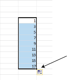
Figure 2–31. The Auto Fill Option button

Click it and you'll see these options:

Figure 2–32. Fill options

The default selection, Fill Series, really identifies what you've just done. If I click Copy Cells, a curiously retroactive thing happens—the initial values, 1 and 3, are simply copied down the range:

Figure 2–33. The Copy Cells option

The Fill Formatting option only copies the formatting associated with the original cells you've copied. Thus if the values 1 and 3 had exhibited a yellow background (we'll see how to do that in Chapter 5: “Formatting Your Data”) selecting Fill Formatting will result in this:

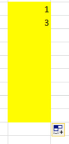
Figure 2–34. Fill Formatting—here, the values aren't filling down the range; only the formatting in the source cells carries over to the selected cells.

The last option, Fill Without Formatting, executes the fill, but doesn't copy the formatting along with it:

Figure 2–35. Fill Without Formatting—only the numerical sequence is carried out, without bringing the formatting along for the ride.

Customizing Auto Fill Lists

Want more? You can also customize an auto fill list, say of friends or clients. That means that if you type one of the names in your customized list and drag it with your mouse, all the other names in the list will appear—just like the built-in days of the week list.

To devise a customized auto fill list:

1. Click the File tab Options Advanced Edit Custom Lists… button: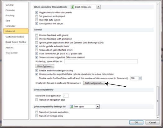
   

   Figure 2–36. The Edit Custom Lists button

2. You'll see the following. Note the four built-in lists we discussed earlier. To start composing your own, just type the names in the List entries area, and press Enter after each entry:
   

   Figure 2–37. The Custom Lists dialog box

3. When you're done, click the Add button. You'll see:
   

   Figure 2–38. Your own custom list

4. Click OK.

Now when you enter any one of those names in a cell (again, it doesn't have to be the first in the list) and drag it with the fill handle, all the other names will appear across a row or down a column, depending on the direction in which you drag, of course. Your friends—and maybe even your boss—will be impressed.

Data Validation: Bringing Quality Control to the Worksheet

It isn't exciting, but data entry is at the heart of every worksheet. The most ingenious, jaw-droppingly-brilliant melange of formulas and charts won't be worth a pixel if the information it works with is suspect, and Excel recognizes that critical point by providing its users with a series of data entry-control, or validation, options that help reduce the likelihood that bad data will compromise your results.

Here's a simple example: Suppose you need to enter the names of states in a range by their two-character abbreviation, the way the post office codes them. You could devise a data validation rule that restricts any data entry in a range of cells to exactly two characters—meaning that if you were to accidentally type CAL instead of CA, you'd be prevented from doing so.

You see the point. By engineering a data validation rule requiring two, and only two, characters in the designated cells your chance of inadvertently making a data entry mistake is narrowed. Of course, our rule wouldn't stop you from erroneously entering NY when you really wanted to type CA, because both have two characters, but it's a start.

So let's try to set up that two-character data validation rule to see how it works.

1. Select any cell and click the Data tab Data Validation button in the Data Tools button group. This sounds strange, but click either the upper half of the button or click the lower half or the small arrow and then click Data Validation. Quirky, but that's how this, and some other Excel buttons, work.
2. Now click the drop-down arrow by Allow in the Data Validation dialog. You'll see:
   

   Figure 2–39. Granting permission: The Data Validation Allow menu lets you decide what sort of data to allow in the selected cells.

3. Click Text length and then “equal to” after you click the drop-down arrow by Data. You'll now see:
   

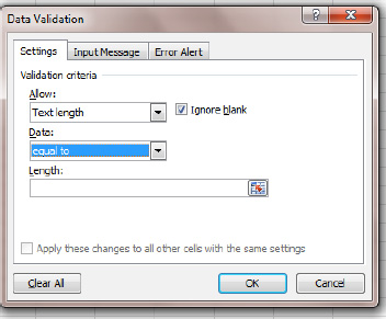
   Figure 2–40 Character test—specifying a two-character data entry requirement.

   NOTE: Clicking the button at the right end of the Length field will temporarily collapse, or shrink, the dialog box when you click it. Collapsing will allow you to see more of the worksheet. Just click the button a second time and the dialog box will return to its original size:

   

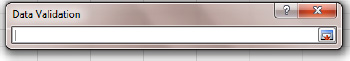
   Figure 2–41. Selected short subject: collapsing the dialog box, an option you'll see in many dialog boxes.

4. Remember—we want to restrict the data in the selected cell to entries of exactly two characters, so just type 2 in the Length field and click OK.
5. Then try to type CAL in your selected cell and press Enter. You should see:
   

   Figure 2–42. Oops—we've typed one character too many.

6. Because we've violated the data validation rule we established—by attempting to enter three-characters—Excel reminds us we can't do it. Either click Retry or Cancel and give it another go, this time restricting the input to two characters. This time, it'll work.

Just keep in mind that by clicking on “equal to” in the Data field we do mean exactly two characters. Entering one character in the cell will also provoke an error prompt. Had we wanted to specify a maximum two characters we could have selected the “less than” data option and typed 3, or “less than or equal to” and typed 2.

But note that Data Validation rules work with a kind of grandfather clause. If you've already entered CAL in a cell in which you then institute a two-character limit, Excel will let the current entry stand. Just don't try typing ARI in the cell now, though.

Once you understand how that example works you can try out some of other data validation options, such as between or greater than; these should now be pretty easy to work out.

And if you want to remove a data valuation rule, just select the relevant cells and click Data Validation Clear All OK.

Making a List—Personalizing a Drop-Down Menu

One of the cooler data validation options is the ability to let you construct your own drop-down menu, from which you can choose from your own list of data. Thus instead of having to type Department names for each employee in our little database, you could batch up something that looks like this, and just click:

Figure 2–43. Fast-track data entry: Drop-down personalized menu

It's easy to devise, too:

1. Enter the items that will populate the menu in consecutive cells. For example, in cells A2:A5 you could enter HR, Marketing, Sales, VP.
   

   Figure 2–44. These names will populate the drop-down data entry menu.

2. Select the range of cells where you want to use the drop-down menu (this is a different range from the one containing the options). That is, you want to select the cells in which the menu will actually appear when you click in any of its cells. In the figure below we'd select the cells in the Department column (you'll see this collection of data again in Chapter 7), but you can really select any column of cells to illustrate the point.
   

   Figure 2–45. These cells will exhibit the drop-down menu.

3. Click Data Validation. Select List in the Allow field.
   

   Figure 2–46. Here's where you select the data that will appear in the drop-down menu.

4. Click in the Source field, and select the range containing the drop-down menu items—in our case =$A$2:$A$5, or whatever range you're using. Note the dollar signs appear automatically when you select the range, because the drop-down menu will likely appear in a whole range of cells—and Excel doesn't want the drop-down source range for each of the cells to change as a result of relative cell addressing (see Chapter 4), i.e., A2:A5, A3:A6, A4:A7. Also remember that if you name the source range—to say Dept—all you need do is type =Dept in the Source field, and that's it.
5. Click OK.
6. The drop-down menu should be ready to go in the selected cells. Just click the drop-down arrow in each cell.

If you change any of the data whose entries appear in the drop-down—say VP to Vice-President—that new phrase will appear in all subsequent data entry using the drop-down menu. But existing records displaying VP won't be changed.

Explaining Data Validation Errors with Error Alerts

Once you've subjected a range to a data validation rule you may want to provide the user with some information about what the rule does. We've already seen that Excel does that by default, by broadcasting the “The value you entered is not valid” message we saw in Figure 2–42. But you can customize that message via the Data Validation Error Alert feature, so that the user is told exactly what sort of data is and is not permitted in the cell. Thus you can compose a prompt that declares: “You must enter two characters in this cell”—and you can also provide an Error Alert that warns the user that the cell entry is wrong, but the cell will accept it anyway if the user wants to go ahead anyway.

There are three sorts of Error Alerts:

• Stop—Excel's default, which blocks entries that violate the data validation rule
• Warning—This notifies the user that the data entry violates the rule, but allows her either to try again or to override the rule
• Information—This one sounds like the others, but it just tells the user the data entry violates the rule—and goes ahead and accepts it

Let's see how to customize a data validation prompt:

1. Select the range of cells to which you've assigned the Data Validation rule.
2. Click Data Validation and click the Error Alert tab.
3. Select the Error Alert type you want to apply from the Style drop-down menu.
4. Type a Title and customized message. For example—if you select the Warning type, you could entitle the message Character Limit, and write: Only two characters permitted in this cell.
5. Click OK.

Once that's done, enter CAL—that is, three characters, and press Enter; you'll see

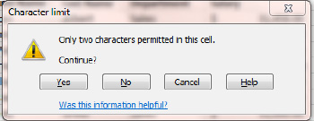
Figure 2–47. Don't say we didn't warn you: A Warning Error Alert. The user will still be allowed to enter three characters anyway.

Note the Continue? prompt, which is supplied by Excel.

Adding Data Entry Instructions with Input Messages

We've seen that Error Alerts tell the user if they've violated a data validation, and what they've done wrong. Input messages tell the user what sort of data is permitted in cells before the data is entered.

To demonstrate how this works:

1. Select that same range of cells with which you've been working.
2. Click Data Validation Input Message. You'll see:
   

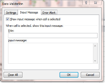
   Figure 2–48. Delivering the message: The Input Message dialog box.

3. Type Two-character limit in the Title field and “You must enter exactly two characters in this cell” in the Input Message field, and click OK.
4. Click in any cell in the selected range; you'll see:
   

   Figure 2–49. Proactive prompt: an input message

The idea is to pre-empt possible data entry mistakes, by letting the user know in advance what's allowed in the cells.

Summary

We've covered lots of ground in this chapter—literally. We've learned how to travel the length and breadth of the spreadsheet and how to introduce data into cells, once we've parked ourselves inside the ones we want, and we've learned how to fend off potential data enty miscues with an array of data validation techniques.

Knowing how to get around the worksheet, select its cells, and post data to them rank among the most essential Excel skills—and as you've seen, they're pretty easy. But sometimes you need to change what you've already done, and in the next chapter we'll see how to go about editing the contents of cells. It's pretty easy, too.