Chapter 3

EditingData

Once you've gotten the principles of data entry nailed down, you'll need to learn about the ways in which you can modify, or edit, the information you've posted to their cells. I'm going to introduce those editing techniques now, because, as someone once said, “Change is good” (when you need to make a change). And when you're working with Excel, it's easy too.

Changing Your Data

Needless to say, there will be times when you'll need to make changes to at least some of the data you've posted to your worksheet. For example, you may have made an error or two, or a data update may be in order. Excel makes editing easy, too, and as usual, presents you with a couple of options.

First and most simply, you can edit the contents of a cell by simply typing over what's already there. If you've entered the number 7 and discover you needed a 77 instead, just select the cell and type 77. Excel overwrites the original number.

However, if you've entered a lengthy expression that contains one small error into a cell, retyping all the contents of the cell for the sake of one correction doesn't seem terribly efficient. For example, say you typed”Now is the time for all good mean,” but you meant men. Again, you could retype the whole phrase, but there are less troublesome ways to get what you want. Here's a more efficient tack:

1. Select the cell.
2. Click in the formula bar, right next to the a you want to remove, as shown in Figure 3–1.
   

   Figure 3–1. Nobody's perfect—I didn't mean “mean.” Note that this correction is being made to the phrase in cell V15.

3. Remember the formula bar—that strip in the upper reaches of your screen that affords you a view of exactly what you entered in the cell. Among other things, the formula bar gives you a place to very easily edit a cell. Here you can click precisely at the place in the phrase you want to change. and do some basic word processing. If you click to the left of the a, press the Delete key once and the letter will disappear. If you click to its right, press Backspace instead.
4. When you've finished your edits, press Enter or click the green check mark, and the edit is completed. Simple!

You can also add text to the cell in much the same way:

1. Click in the formula bar at the appropriate point in the text and just type. As with Word, the text will push the adjoining words aside.
2. Then press Enter or click the green check.

You can also edit data in a cell by deploying an ancient spreadsheet keystroke: the F2 key. Here, instead of clicking inside the formula bar, click the cell and press F2. The cursor will be placed at the end of text, as shown in Figure 3–2.

Figure 3–2. Using the F2 key to get inside the cell

Once the cursor is in the cell, you can press the left arrow key to make your way back to that surplus a. Once you're there, just backspace or delete, and then press Enter, and the deed is done.

Note as well that when you start to edit cells, the mode indicator lurking in the lower left of the status bar changes, as shown in Figure 3–3.

Figure 3–3. The Edit mode indicator turns on when you begin the cell-editing process.

Undoing an Edit

There's yet another way to revise the contents of your cells, though you might not think of it as an editing command—it's the Undo button, stored in the Quick Access toolbar (shown in Figure 3–4).

Figure 3–4. The Undo button

By clicking that button (or utilizing its keyboard equivalent, Ctrl+Z), you can nullify the command you've just executed (note that a small number of commands can't be undone, such as adding a new worksheet to the workbook). Moreover, if you click Undo repeatedly, each previous command will be repealed in succession. And if you click the small drop-down to the right of Undo, a history of the commands you've carried out this session will be shown on the screen, something like Figure 3–5.

Figure 3–5. Long memory: The Undo drop-down menu

Drag your mouse through those commands you want to undo, as shown in Figure 3–6. Click your mouse, and those selections will be undone.

Figure 3–6. Choosing which commands to undo

Undoing What You've Just Undone with the Redo Button

There's a flip side to the Undo command, too: Redo, represented by that right-curling arrow just to the right of Undo, as shown in Figure 3–7.

Figure 3–7. Having second thoughts? Undo the undos with Redo.

When clicked (keyboard equivalent: Ctrl+Y), Redo can undo your undos, if that's not too discombobulating. That is, if you execute an undo and instantly regret it, then click Redo and that undo will be forgotten. And as with Undo, Redo also sports its own history via a drop-down menu (revealed by clicking the little arrow to the right of the Redo button), recording the commands you've undone. It works the same way as the Undo drop-down.

Deleting Cell Contents

Of course, the most dramatic way to edit a cell is to delete its contents—and if that's what you want to do, just select the cell and press the Delete key. But bear in mind that if you want to delete agroup of cells, select them by using one of the methods already described in Chapter 2, and then press Delete, as shown in Figure 3–8.

Figure 3–8. First select the range of cells, and then press Delete.

Copying and Moving: Duplicating and Relocating Your Data

There will be times—probably many times—when you'll want to make a copy of a range of data. The basic means for doing so are pretty basic and easy, and resemble the ways you'd carry out the process in Word. At other times you'll want to move a range—an equally easy process that also goes under the storied name of cut-and-paste.

Copying Data

As usual, Excel presents the user with several ways in which to copy data, but we'll start with the textbook approach. To copy, do the following:

1. Select the range you wish to copy.
2. Click Home tab, and choose Copy from the Clipboard button group (see Figure 3–9).
   

   Figure 3–9. The Copy button

3. Your range will be surrounded by what are called marching ants (really), those animated dashes trooping around the range (see Figure 3–10).
   

   Figure 3–10. On the march: The ants are part of the copy process.

4. Click in the first cell of the destination range—that is, the area in the worksheet to which you want to paste the copied data (see Figure 3–11).
   

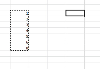
   Figure 3–11. You only have to click in the first cell of the destination range.

5. Click Home, and then click Paste in the Clipboard button group (see Figure 3–12).
   

   Figure 3–12.. The Paste button

You're done (see Figure 3–13). The keyboard equivalents for copy and paste, by the way, are Ctrl+C and Ctrl+V, respectively.

Figure 3–13. The destination range receives all the copied cells.

To summarize, the copying process asks you to select what it is you want to copy, and then to indicate where the copy is going to be pasted on the worksheet. Note that when you paste, you need only click in the first cell of the destination range, because Excel is smart enough to know that if you're copying 12 cells, you're going to paste 12, too (see Figure 3–14). And note there's another keyboard equivalent to Paste available in this context—pressing the Enter key.

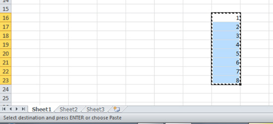
Figure 3–14. The first cell in the destination range determines where the rest will be pasted.

Moving Data

Moving data isn't much different from copying and pasting it. Select the range, but this time click Home Cut (see Figure 3–15). The keyboard equivalent for cut is Ctrl+X.

Figure 3–15. The Cut button

Note that, curiously, clicking Cut doesn't cause the range to disappear from the screen immediately; the data stays there until you click in the first cell in the destination range and then click Paste (or press Ctrl+V). Only then does it get uprooted from its original position and move to its new range.

The Clipboard: The Storage Area for Copied and Cut Data

By now, you may have taken note of the button image characterizing the Paste command: a clipboard, in the Clipboard button group (see Figure 3–16).

Figure 3–16. The Paste button

The image alludes to an area in Excel's brain, naturally enough called the Clipboard, in which data that you've copied and/or cut is stored until you decide to paste it. The Clipboard can warehouse up to 24 different copied or cut items, all of which can be pasted to your worksheet when you wish. To see what I mean, let's try it out.

1. On a blank worksheet, type the text shown in Figure 3–17 (i.e., the text in cells C9:C12 and the values in cell I11:I13.
   

   Figure 3–17. The Fab Four and three values

2. Then click the dialog box launcher in the Clipboard button group. That's the small arrow by the Clipboard title, as shown in Figure 3–18.
   

   Figure 3–18. The Clipboard dialog box launcher

3. The Clipboard dialog box will appear, as shown in Figure 3–19. Select the text in cells C9:C12.
   

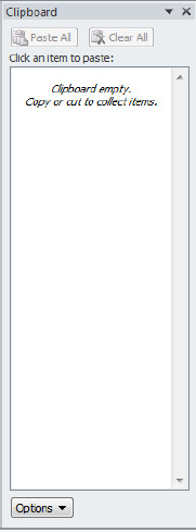
   Figure 3–19. The Clipboard area

4. Click Copy, and the text shown in Figure 3–20 will appear in the Clipboard area.
   

   Figure 3–20. Your copied text, stored and ready to paste

5. Then immediately select the values in cells I11:I13, and copy them as well. The Clipboard should now displays what's shown in Figure 3–21.
   

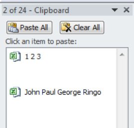
   Figure 3–21. Your choice: You can paste either—or both!

The Clipboard now records two entries, either one of which can be pasted by simply clicking in a destination cell and then clicking the Clipboard item you need.

Note as well that by clicking Clear All you can empty the Clipboard, and by clicking the X in the Clipboard's upper-right corner you stop it from being displayed.

Summary

Once you build up your data entry and editing chops, you'll want to start learning about the ways you can do something with the data—that is, writing formulas and using other means for gleaning something new from the information you've posted to the workbook. Entering test scores is one thing; but calculating a test average—ah, that's what Excel's about. Just turn the page.