Chapter 10

Printing Your Worksheets: Hard Copies Made Easy

We hear about the paperless office all the time, but just cast a glance at your office or your desk at home—lots of paper still out there, no?

That's the reality, of course. Sooner or later, you'll be called upon to commit your spreadsheet data to printed form—for distribution at meetings, or for handing in to instructors, or for inclusion in booklets and brochures.

Once you get to it, you'll find printing in Excel to be pretty simple—as it should be. In some ways it's almost self-evident, meaning that with just a bit of exposure to the feature you'll probably be able to figure out a good deal of what you need to know by yourself. And as usual, Excel gives you more than one way to carry out many of the basic printing tasks.

Deciding What You Want to Print

The first consideration in printing the data on your worksheet is how much of it you want to print. Your intention may be simple: to print everything on the sheet, and that makes your job easy. On the other hand, you may want to print just part of the data, but that objective only makes the job slightly harder.

Printing the Entire Worksheet

Let's say that for starters you want to print all the data on one worksheet (not the entire workbook, though). To illustrate, enter the values from Figure 10–1 in cells C9:D13.

Figure 10–1. Fit to print: Ten cells worth of data

The next step is to access the Print command sequence, either by clicking the File command tab and choosing Print, or by calling upon the venerable Ctrl+P keyboard shortcut. Either way, you'll be brought to the Backstage (see Figure 10–2).

Figure 10–2. A visit backstage: Your print options (at least most of them). Note the Print button.

Note the large print review pane to the right. In the simplest-case scenario, all you have to do now is click the large Print button and head for your printer to collect your copy.

OK, it isn't always quite that easy, but it usually doesn't get much more challenging than that. To delve into something slightly more complex than printing a worksheet, let's first see how to print a selection.

Printing a Selection

Let's call up that Student Scores workbook, in which all those bonus grades were handed out. The data there was stored in the range J7:L12, and now we want to print the contents of just that range (see Figure 10–3).

Figure 10–3. Those student scores again, this time to be printed

First, delete any charts you may have on the sheet. Again, you can activate the Print command, but this time you'll see the screen shown in Figure 10–4.

Figure 10–4. Probably not what you had in mind. There are the names, but where are the grades? Note the Print Active Sheets option.

Well, that's not terribly satisfactory, is it? All we're seeing are the student names, which aren't accompanied by their grades. Note as well the legend at the bottom of the screen that states 1 of 2, referring to pages; if you click the arrow to the right of the number 2 to travel to that page, you'll see what's shown in Figure 10–5.

Figure 10–5. There are the scores, but not where we want them.

So what's going on? Really, two things:

• When you instruct Excel to print a worksheet, it searches by default for data by proceeding from the beginning of the sheet (i.e., the A column), and will include all the blank areas it finds en route to the data until it actually finds the data. It'll thus print this worksheet starting at column A up to and including the area containing the data, starting in the J column.
• The Print Active Sheets option will also print everything on the sheet, no matter where that data is located.

For sake of the illustration, this means that if you had devised a worksheet whose data starts in the X column, Excel would by default print columns A through W—all of these blank—before reaching the actual data to print, meaning you'd end up with a collection of empty printed pages before the page you wanted to print rolled out. It also means that if you have a small range in A7:B19 that you want to print, and you also happen to have squirreled away a bit of data in cell ZA241, Excel will by default print all the blank columns between B and ZA too, until it finally stops at ZA241.

But all that happens by default, when you simply click the Print button without giving any additional thought to what you wanted to see on paper, and leave the Print Active Sheets option selected. And that default makes sense if you've started your data entry in the A column and have a confined range of data to print, as is often the case.

But it doesn't make sense in our case, where we'd end up with a two-page printout, with the student names on one page and their grades on another.

Needless to say, there's a way to deal with our little problem—by selecting precisely the range you do want to print and then telling Excel to print only that area. You do that by selecting the range (in our case J7:L12), and then returning to the Print dialog and clicking Print Selection, thus overruling the default Print Active Sheets option (see Figure 10–6).

Figure 10–6. Printing only want we want to print: Choosing the Print Selection option

Once you've clicked that option, you'll see what's shown in Figure 10–7.

Figure 10–7. All the data is on one sheet now, and the print output will only require one page.

Thus, in order to print some, but not all, of the data on a worksheet, you just select the desired range, activate the Print command, and select the Print Selection option. Then just click Print.

Surveying Printing Options: The Print Backstage

Now let's take a closer look at the various options you'll encounter when you enter the Print section of the Backstage (see Figure 10–8; also see the Quick Start Guide for a reminder of what the Backstage is).

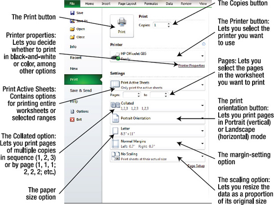
Figure 10–8. The various Print options in the Backstage

Again, many of these options are easy to figure out on your own:

• The Print button actually executes the print when clicked.
• Copies allows you to set the number of copies you want to print.
• The Printer button lets you select the printer to which you want to print, if you have access to more than device. Clicking the Printer drop-down arrow reveals a menu enabling you to click the printer to which you want to direct the print (see Figure 10–9).
  

  Figure 10–9. Just select the printer you want to use.

• Print Active Sheets, as mentioned, is the default option for this command, and offers the selections shown in Figure 10–10. You can elect to print the entire workbook—that is, all its sheets—or just the range you've selected (Print Selection). The reference to Print Active Sheets (in the plural) means that if you've grouped two or more sheets, their data will be printed.
  

  Figure 10–10. These options allow you to choose what segment of the workbook you want to print.

• Pages lets you decide which pages on the worksheet you want to print. If you print a large swath of a workbook, the overall print area may be too large to capture on one page, so Excel will need to print additional pages, as in our student grades printout before we selected a specific range to print. When multiple pages are required, the page boundaries are represented in the workbook by dotted lines, which appear once you've viewed the imminent printout in the Backstage (see Figure 10–11).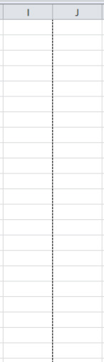
  

  Figure 10–11. The dotted line indicates where a new page will begin in a printout.

• The Collated option only applies if you're printing at least two copies (see Figure 10–12).
  

  Figure 10–12. The Collated and Uncollated options

  By default printouts are collated, meaning that if your output will consist of three pages, the pages will appear in sequence (e.g., 1, 2, 3 and 1, 2, 3 again). But if you select Uncollated, all the page 1s will print first, followed by all the page 2s, and so on. You might want to use the Uncollated option if you need to make some hand-entered corrections on all page 3s, for example.

• Orientation gives you two print options: Portrait and Landscape (or vertical and horizontal, respectively). Landscape orientation is commonly used for printouts that contain many columns of data and would spill across multiple pages if they were they printed in Portrait mode.
• The paper size option lets you select the size of paper with which you're working. Obviously, paper size will affect how and where the data gets distributed in a printout (see Figure 10–13).
  

  Figure 10–13. Sizing up your printouts with the paper size option.

• The Margins option is easy to overlook, but it's important because Excel printouts have to work with page margins. Excel's default margins (called Normal) stand at .7 inches left and right, and .75 top and bottom (see Figure 10–14).

Figure 10–14. Print margin settings

You can select any of the recommended settings shown, including the Custom Margins… option, which sits at the base of the menu. Clicking that choice presents you with the Margins tab in the Page Setup dialog box (see Figure 10–15).

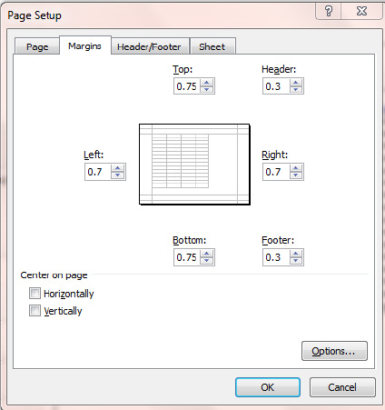
Figure 10–15. Where you can customize print margins

Just type the desired margin(s) and click OK.

Note the Center on page option. Clicking both Horizontally and Vertically will position the data you want smack-dab in the middle of the page. Recall that our Student Scores print preview indicated that the scores would be printed in the upper-left corner of the page (see Figure 10–16).

Figure 10–16. The student scores: Ready to print, but leaving a great deal of white space on the page

Select both Center on page options and the printout will be redesigned, as shown in Figure 10–17.

Figure 10–17. It's still not a museum piece, but the data is now centered both horizontally and vertically.

• The scaling options (see Figure 10–18) allow you to modify the size of the data to be printed—not by directly changing the font, but rather by refitting the data on the page so as to tidy the results.
  

  Figure 10–18. Economy of scale: The print scaling options

Here's a classic example: you need to print data consisting of many columns, and the print preview reveals that the last column is going to have to be shunted to a second page, because the first page has simply run out of room. And that's messy. By selecting Fit All Columns on One Page, Excel will slightly downsize all the data on the printout so that the renegade column will be able to join the other columns on the first—and what is now the only—page.

Setting the Print Area

In addition to the printing capabilities you'll find in the Backstage, there are some additional and important options stored in other areas of the worksheet. You've already seen that by selecting a specific range to print, you can avoid the problem of overprinting (i.e., printing blank areas of the worksheet that you don't need to see in your printed results). But selecting a print range may cause a problem or two on its own, because once you select that range you need to print it right away. If you decide you want to work elsewhere in the sheet before printing, you'll have to click elsewhere to begin your work, which will deselect the range you want to print.

But Excel lets you have it both ways by letting you designate and save a print area so you can go on do to work somewhere else before printing.

---

To see how the Print Area option works, select the student grades and click the Page Layout contextual tab, and then click Print Area Set Print Area in the Page Setup button group (see Figure 10–19).

Figure 10–19. Setting the print area

---

You'll see a dotted-line border surrounding the area you've chosen to print, which will remain in place even if you click somewhere else on the worksheet (see Figure 10–20).

Figure 10–20. The print area is designated by the dotted-line boundary.

Now whenever you're ready to print, just return to the Backstage and click that large Print button.Justmake sure you don't select Print Selection at the point of actual printing though, because if you do, anyrange you happen to have currently selected will be printed instead of the print areayou designated. Click Print Active Sheets or Print Entire Workbook instead. If you save the document, the print area will be saved, too. To clear the print area, click the Page Layout contextual tab, and then click Print Area Clear Print Area in the Page Setup button group.

Customizing Your Printing

In addition to the Print Area button, several other useful print-related options are scattered among Excel's ribbon tabs. The Page Layout tab contains a number of buttons that emulate many features available in the Backstage (see Figure 10–21).

Figure 10–21. The Page Layout tab

Working with Page Breaks

The first three buttons on the Page Layout tab—Margins, Orientation, and Size, provide alternative ways to access the same trio of options in the Backstage; their menus are identical to the ones shown earlier (see Figure 10–22).

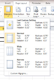
Figure 10–22. Look familiar? You'll see the same menu when you work with margins in the Backstage.

But the button to the right of Print Area (Breaks; see Figure 10–23) does something different.

Figure 10–23. Those are the breaks: Where to establish a page break

Click the arrow beneath the Breaks title and you'll see the options shown in Figure 10–24.

Figure 10–24. The Insert Page Break option

What does inserting a page break do to your printout? Well, first consider what Excel does by default. When you execute a printout, Excel prints as much of the data as it can on the first page, until it runs out of space. It then goes on to print additional pages if it needs them. But what the Insert Page Break option does is let you produce a second page earlier than necessary; that is, before a second page would naturally have to be printed.

For example, recall the PivotTables workbook, spanning the range A1:D17 (we had added one record in the course of our exercise). Open that workbook and survey the data. Because the data encompasses only 17 rows and starts in the A column, we'd only require one page to print it all (see Figure 10–25).

Figure 10–25. Only one page required

But let's say that you needed a new, second page, starting with Dodsworth's sales record. If that's what you want, click in cell A9—where Dodsworth's record starts, and click the Insert Page Break command. You'll see the data shown in Figure 10–26.

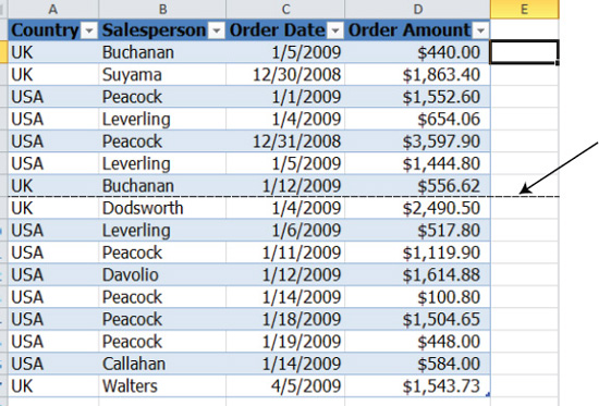
Figure 10–26. Note the dotted line, which signifies where the second page will start.

Now your printout will result in two pages. If you decide to reconsider this two-page motif, you can remove the page break by clicking the worksheet where you've instituted the break (in row 9, on Dodsworth's record), and clicking Remove Page Break—the option which appears right beneath Insert Page Break on the Breaks button. Doing so will return you to the original one-page printout.

Previewing the Page Break: Getting a Bird's-Eye View of the Printout

If the data you want to print contains many records and will likely result in a multipage print, or if you've inserted your own page breaks as illustrated previously, you may want to get a global idea of how the printout will look in its entirety. Realizing that the normal worksheet view may not be able to display all the data at one time without you having to scroll down and/or across repeatedly, Excel offers a page break preview, which presents the printout-to-be in a curiously miniaturized form (see Figure 10–27).

Figure 10–27. The page break preview: The two-page salesperson printout, with the page break inserted by Dodsworth's name

Note the watermark-like Page 1 and Page 2 indicators, superimposed on the data. The page break preview does two things:

• It shrinks the print preview so you can see all, or at least considerably more, of the data on one screen.
• It lets you move the current position of the page break.

To illustrate, in the PivotTables workbook, click the View contextual tab, and then click Page Break Preview in the Workbook Views button group (make sure the page break by Dodsworth's name is in place) (see Figure 10–28).

Figure 10–28. The Workbook Views button group

Figure 10–29. Another Page Break Preview button

After clicking Page Break Preview, click OK on the introductory dialog box, and you'll see the preview shown in Figure 10–30.

Figure 10–30. Getting the big picture with the page break preview

Again, because the view of the data is scaled down, you'll still be able to see many if not all of the records in a large set of data in one glance.

In addition, note the solid blue line demarcating Page 1 and Page 2. You can click and drag that line if you want to readjust the point at which the second page begins.

To illustrate, say you want to move the page break to a position above Peacock's record in row 11. Click the blue line and drag it down two rows, as shown in Figure 10–31.

Figure 10–31. You can click when you see the double-sided arrow, and then drag.

Then release the mouse. You'll see the display shown in Figure 10–32.

Figure 10–32. The newly designated page break

Note, by the way, that if you have a lengthy collection of records and you examine it in the page break preview, you'll see dotted lines instead (see Figure 10–33).

Figure 10–33. An excerpt of a larger set of records as portrayed by the page break preview

The dotted line here represents a natural page break—that is, the point where the page simply runs out of room and has to continue the data on a next page.

When you've completed your visit to the page break preview, you can restore the basic default view of the worksheet by clicking the View contextual tab, and then clicking the Normal button in the Workbook Views button group.

Printing Titles

Returning to the Page Setup group, you'll find another button that deserves your attention: Print Titles (see Figure 10–34).

Figure 10–34. The Print Titles button

Print Titles offers one way to resolve another one of those classic spreadsheet issues—one already discussed in a slightly different context. If you print a long set of records topped by a header row, that header row will print, naturally, but it'll only appear on page 1. And if you need to print a page 2, 3, and so on, these pages won't display the header—at least not by default.

But Print Titles offers a kind of a Freeze Panes command for printing (seeChapter9). Just as Freeze Panes keeps designated rows or columns on the screen even as you scroll away from them, Print Titles allows you to print header rows (or columns) on every page of a multipage printout, reminding you which data is stored under which heading.

To illustrate, printing this worksheet with 800 rows of data will display the header row on page 1 only, at least at the outset (see Figure 10–35).

Figure 10–35. Pages 1 and 2 of a lengthy printout: The header row appears only on the first page

As a result, you may not be able to easily tell on page 2 which data is associated with which heading.

And that's where Print Titles comes in.

1. To try it, go back to the PivotTables workbook and make sure you've kept that page break in the row right above row 11. In the Backstage print preview, you'll see two pages (see Figure 10–36).
   

   Figure 10–36. Again, the header row only displays in page 1.

2. Click the Page Layout contextual tab, and then click Print Titles in the Page Setup button group. You'll see the dialog shown in Figure 10–37.
   

   Figure 10–37. The Sheet tab of the Page Setup dialog box

3. In the Rows to repeat at top field, just click anywhere in row 1 on the worksheet. You'll see what's shown in Figure 10–38.
   

   Figure 10–38. Row 1 will now print at the top of every page.

4. Click OK, and return to the Backstage print review and look at the two pages (see Figure 10–39).

Figure 10–39. Now page 2 also exhibits the header row.

Now every page will display the header row, no matter how many pages are required by the printout.

Adding Headers and Footers

There's still another way to engineer your printout so that the same text appears at the top (or the bottom) of every page: by adding a header and/or footer. As with Word, headers and footers feature recurring text on every printed page, such as the name of the designer of the spreadsheet, the current page number, the date on which the worksheet was printed, or really anything you want to see there.

Now, introducing headers and footers into a printout may trigger a question: Doesn't the Print Titles feature just discussed do the same thing that headers do—namely, repeat some selected text across the top of every page?

The answer is, sort of. It's true that the Print Titles select-a-row selection and page headers both emblazon the tops of printed pages with text, but there's a difference: the Print Titles option grabs its data from rows on the actual worksheet, while header and footer data is entered in a separate area external to the worksheet, so it won't be found in any cells. Thus, you'll never see header data in A1. If you do want to see the data in row 1 at the top of each page, use Print Titles.

Adding Headers and Footers in the Page Layout View

As usual, there are a couple of ways to compose a header or footer. One is to enter it in the Page Layout view, which offers another way of viewing a worksheet; it's accessible via the Workbook Views button group (see Figure 10–40).

Figure 10–40. Where to find the Page Layout button.

Click that button while in the PivotTables worksheet and you'll see the screen shown in Figure 10–41.

Figure 10–41. How the salesperson data looks in the Page Layout view. This is page 1.

The Page Layout view attempts to portray your data exactly as it will print. Note the narrow space representing the physical edge of the page (by the arrow), and the ruler atop the page, indicating the dimensions of each column.

You can enter headers and footers in this view. Note the “Click to add header” area; resting your mouse there reveals three subsections: a left, center, and right area, each of which turns blue when your mouse is poised atop it (see Figure 10–42).

Figure 10–42. Click where you see the blue tint and simply start to type; the header will appear there.

Click in any or all of the three blue areas and type whatever text you want. You can also scroll to the bottom of the page to the “Click to add footer” caption, which works the same way (see Figure 10–43).

Figure 10–43. Three headers, one each positioned in the left, center, and right header areas

Once you've typed in your text, each header will appear at the top of every printed page.

Adding Headers and Footers Using the Page Setup Dialog Box

You can take another route to adding headers and/or footers via the Page Setup dialog box, which you can access directly by clicking the Page Setup dialog box launcher (see Figure 10–44).

Figure 10–44. Clicking the dialog launcher button brings you to the Page Setup dialog box.

Once you've clicked to activate the dialog box, click its Header/Footer tab. You'll see the screen shown in Figure 10–45.

Figure 10–45. The Header/Footer tab. Note that the header data entered in the previous exericise is visible.

The header information entered previously is still visible, but if you click the arrow by the header field, you'll see some additional, built-in header options (see Figure 10–46).

Figure 10–46. Built-in header options. You'll see the same choices if you click the arrow in the Footer field.

Among other things, these selections will record the page number in the header, or a Page 1 of x option, which notes the current page number relative to the total page printout count. For example, the header on page 1 of a three-page printout would read Page 1 of 3. Other built-in options provide the user's name and the date on which the print was executed in the header/footer.

Adding Custom Headers and Footers

You can access even more header/footer options by clicking the Custom Header and Custom Footer buttons (see Figure 10–47), though most of these really just offer equivalents to the options already discussed.

Figure 10–47. Where you can access additional header and footer options

Click Custom Header and you'll see the dialog shown in Figure 10–48.

Figure 10–48. The Custom Header dialog box

Here you can see three edit boxes, or sections, which correspond to the three header areas (that turn blue) in the Page Layout view. Note the existing header data lurking behind all those button descriptions, too. This text can be deleted in word-processing fashion: just select the relevant header and press the Delete key.

You can click in any one of the edit boxes and type any header data you wish, and you can click any of the buttons above the edit boxes to access additional options. The following list reviews what these buttons do (from left to right):

• Format Text: Clicking this button will call up Excel's standard Font dialog box, enabling you format header text.
• Insert Page Number: This button posts a page number on each printed page.
• Insert Number of Pages: This places the total number of pages in a printout in each page's header/footer. Thus, in a three-page printout, a 3 will be displayed on each page.
• Insert Date: This records the date on which the printout was executed. This means of course that the header/footer will change according to the date on which you print.
• Insert Time: This displays the time when the printout was issued.
• When you click one of these buttons in the desired section, a strange-looking code is installed in that area. For example, if you click the Insert Date button in the right edit box, you'll see what's shown in Figure 10–49.

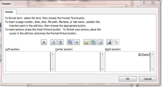
Figure 10–49. Inserting today's date in the header, whatever today's date happens to be

Click OK and you'll be returned to the Header/Footer tab, where you'll see the date previewed (see Figure 10–50).

Figure 10–50. The date displayed on the Header/Footer tab

Click OK again and the date header will be incorporated into the printout.

• Insert File Path: This lists both the workbook name and the folder(s) in which the workbook has been saved (e.g., C:UsersAbbottDocumentsPivotTables). This option is widely used in the corporate world, because it informs viewers of the workbook where it is stored in a network.
• Insert File Name: This just prints the name of the workbook (e.g., PivotTables).
• Insert Sheet Name: This prints the name of the worksheet whose data is being printed (e.g., Sheet1, or any customized name).
• Insert Picture: A rather exotic option, this lets you position a photo or clip art in the header/footer, such as a company logo. The dimmed button to its right is Format Picture, which contains options enabling you to modify that picture.

Printing the Gridlines and Headings

Another pair of options you'll find in the print repertoire let you print both the gridlines that border every cell in the worksheet and the row and column headings themselves—the actual numbers and letters that identify cells by their addresses.

Both are easy to do, and the options are alongside one another in the Sheet Options button group on the Page Layout contextual tab (see Figure 10–51).

Figure 10–51. The Print Gridlines and Headings options

Checking the Print box of the Gridlines option will print the lines around every cell selected for printing. This option is not identical to drawing lines around cells with the Borders command in the Font button group. That latter option allows you to select exactly those cells around which you want to see borders. Print Gridlines, however, will automatically print gridlines around all the cells in your printout.

Thus, if you select the range to print shown in Figure 10–52 and click the Print box of the Gridlines button, the results will look like Figure 10–53.

Figure 10–52. Six cells selected for printing

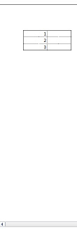
Figure 10–53. The gridlines around each cell will print. No borders have been drawn around the cells.

If you click the Print Headings (that's Headings, not Headers) option, you'll see something like Figure 10–54, for example.

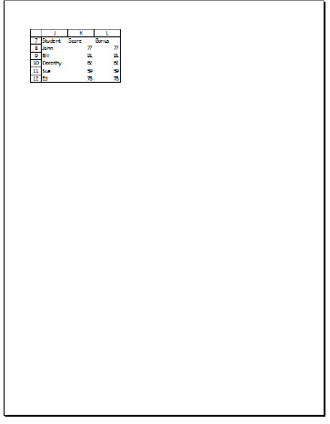
Figure 10–54. Printing row and column headings

You might want to print headings when you want viewers of the printout to see exactly which cells contain particular data.

Summary

As stated at the outset of the chapter, printing is generally a simple task: select the range you want to print and print exactly that selection, or set the print area and print. The embellishments—printing titles at the top of your pages or headers and/or footers—are simple too.

Now that you've learned how to convert your data to hard-copy form, we're going to return to Excel's native electronic environment and talk about macros, which provide a surprisingly easy way to automate tasks you'd just as soon have someone else do. And that someone else is Excel