Chapter 7

Sorting and Filtering Your Data: Excel's Database Features

You hear the term database all the time, even in everyday conversation, but the concept is rarely defined. People tend to rely on a common sense understanding of databases, and that's usually good enough—and the reality is that even Excel has found the task of deciding what it really means by databasea bit troublesome. That doesn't have to concern us, but on the other hand, since we need to use the term throughout this chapter, we'll plunge ahead and define a database as a collection of records (i.e., rows) organized into fields, all of which are topped by titles.

And as it turns out, that's pretty close to the common sense understanding. Thus, the very standard collection of data shown in Figure 7–1 would qualify as a database.

Figure 7–1. A garden-variety database

Pretty standard, no? Note that the first row—called a header row—contains the titles of each field, or column. And it doesn't matter if the database contains 30,000 records or 3. Either way, it's a database.

Databases serve as the starting point for many of the tasks users can carry out in Excel. For starters, databases can be sorted, either in numerical or alphabetical order, and either ascending or descending—that is, A to Z, or Z to A, or 1 to 100, or 100 to 1. And the same can be done with dates that you want to sort in chronological order, because remember, dates are values.

In addition, users can pose all sorts of questions of databases, such as

• How many people work in HR?
• What's their average salary?
• How many people in the company make more than $50,000?
• How much money did each salesperson earn each month?

In order to answer these questions, databases can be asked to produce a subset of their records—that is, only those records that meet a certain criterion or criteria that the user establishes. Excel offers a range of ways in which these kinds of questions can be asked—and answered—and we'll look at some of them in this chapter.

And because databases depend on accurate data entry, Excel provides a set of controls on the data entry process, through which the user can at least minimize the likelihood of making mistakes. Called data validation techniques (introduced previously in Chapter 2), these are fast and easy ways to place limits on the kinds of data that can be entered in cells. You'll learn about some of these too. But first, let's take a look at sorting.

Sorting Data: Instilling Order in Your Data

When I did my thing as a corporate trainer in New York, our in-house training manuals described sorting as an advanced topic. It isn't. Spreadsheets nowadays make the job of arranging values and/or text in order an easy task. Here's an example:

1. Enter the records from Figure 7–2 in a blank workbook, starting at cell H7 (note the header is formatted differently from the rest of the database; this will be important later).
   

   Figure 7–2. Out of sorts: Our workforce, ready to be sorted

2. Save the workbook as Sort. Note that the first and last names have been assigned separate fields; this is a good thing to do when working with databases.
3. Now let's suppose we want to sort this database by the last names of the staff. Start by clicking anywhere in the Last Name column. Don't try to select the entire database; that's totally unnecessary at best and will cause problems at worst. Then click Home Sort & Filter in the Editing button group. You'll see the drop-down shown in Figure 7–3.
   

   Figure 7–3. Where to start sorting

4. Click Sort A to Z, and you'll see the content shown in Figure 7–4.

Figure 7–4. All done!

That's it. The last names are sorted in A-to-Z order, and the deed is done.

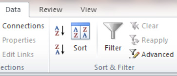
Figure 7–5. Sort of the same: Another set of sort buttons

Any questions? You may well have a few. To answer one right away: Yes, when you sort by a field, all the other fields in the database get sorted too, so that all the data fields will continue to be aligned with each other. Thus, Zachary will still lined up with Quincy; he won't be randomly paired with someone else's first name.

Another question might involve the header row, which remains in position. Why wasn't that row sorted along with the others? How does Excel know that the phrase Last Name really doesn't signify someone's last name?

There are two answers to this question:

• Excel won't sort the first row in a database if it's formatted differently form the other database rows.
• In addition, Excel won't sort a top row if there's a data type disparity somewhere in the database. That means that if a heading in the database is text and the cells beneath it consist of values, Excel assumes the heading is just that—a heading, not data—and is not to be sorted. As you can see, there's a data-type disparity in our database—in the Salary field.

Once you understand how sorting works, you should be able to sort any field in either direction. Thus, if you want to sort salaries in descending order, just click anywhere in the Salary range and click Sort Largest to Smallest on the Sort & Filter drop-down menu. And yes, we've just seen something new. When Excel recognizes a field filled with values, it converts its sort options into the largest-to-smallest variety. Sort a text field and Excel presents you with its A-to-Z choices instead. Just note that if you happen to click the header cell of a value field that happens to be text (e.g., Salary), the drop-down will state Sort A to Z, even though the actual data consists of values.

Sorting by Two Fields: The Hows and Whys

Consider this scenario: you're the instructor of a large, lecture-hall-sized class, and you've entered the names of all your students on a worksheet. You want to sort them in the standard last-name alphabetical order, but a quick scan of the data turns up several students with identical last names. You'd then probably want to sort the first names as well, so that Edna Arnold will appear in the sort before Gary Arnold.

And that introduces a classic sorting issue. Sorting by a second field is something you may want to do when, and only when, you have duplicate data in the first field—that is, when you discover at least two entries in that field with the same contents. There's simply no point in sorting by a second field unless you have duplicate data in the first.

And as it turns out, our own database exemplifies this point. Suppose we want to sort our records by department. The Department field exhibits numerous duplicates, so we could sort by a second field as well—say, salary. In other words, we want to wind up with the results shown in Figure 7–6.

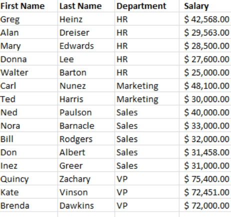
Figure 7–6. Tilling two fields: Sorting by Department and Salary

Note that Department is sorted in A-to-Z sequence but Salary is sorted largest to smallest—kind of the opposite direction—because we wanted to see who were the highest earners in each department. And how do we do all this? Here's how:

1. First click in the first field by which you want to sort. You need to decide which field gets sorted first. In our case, we want to sort the Last Name field first, and then Salary, so click in the Last Name field.
2. Click Home Sort & Filter Custom Sort, and you'll see the dialog shown in Figure 7–7.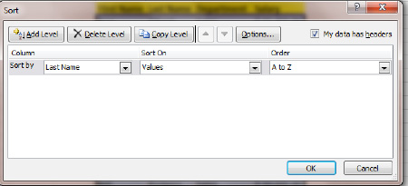
   

   Figure 7–7. The Sort dialog box

   NOTE: The Sort by field is filled with Last Name, because that's the field in which we click to start the process. If you click in the wrong field by mistake, you can just click the accompanying drop-down arrow, which lists all the fields in the data base. Note in addition the Order field displays A to Z, the default sorting option selected by Excel. If you want to sort the field as per the Z-to-A ordering, click the drop-down arrow and select that option (there's a bit more to say about the other Sort On options; we'll get to that a bit later).

3. We want to sort by two fields—so where's the second one? Click the Add Level button, and you'll see a second entry beneath the Column entry, entitled Then by.
4. Click the drop-down arrow and click Salary, the second field by which we want to sort (see Figure 7–8).
   

   Figure 7–8. The second sort field comes into view.

   NOTE: By default, Excel checks the My data has headers check box, thus telling the application not to sort the first row in the database.

5. Now that we've added the second field to be sorted, we need to look at Order, which reads Smallest to Largest. Click that down arrow and select Largest to Smallest, the direction in which we want to sort Salary.
6. Click OK.

You can also click any field in the dialog box and click Delete Level if you decide you want to remove it as a sorted field. The up and down arrows alongside the Copy Level button allow you to promote or demote fields in the sort order. Thus, if you wanted to sort Salary first you'd click in that field and then click the up arrow. Salary will move above Department in the dialog box and be sorted first.

Sorting by Cell Format

Now what about those additional options on the Sort On drop-down menu—namely, Cell Color, Font Color, and Cell Icon? These are choices you're far less likely to select; they relate to conditional formatting, allowing you to tell Excel to sort cells (or the text in them) that have been, for example, formatted green before cells that have been formatted red.

Thus, if you were to click Cell Color, additional buttons asking you to identify which color is to be sorted first would appear in the dialog box; or in the case of Cell Icon, which conditionally formatted icon would receive sorting priority (see Figure 7–9).

Figure7–9. Two different sorts of sorts based on conditional formats (the first by cell color and the second by cell icon)

Finding What You Want with Filters

In the introduction of this chapter I pointed out that a great deal of the work people do with databases involves asking questions of a database's records; questions whose answers are usually supplied by just some of the records—such as which people in the company earn more than $50,000, or who works in the Sales department. Excel offers a very easy way to ask and answer these kinds of questions—through its filter feature.

Filters have been around in Excel for quite some time, but they've been improved, without compromising ease of use—as you're about to see.

1. To begin filtering your data, just click anywhere in your database, and then click the Filter button in the Data tab's Sort & Filter button group (see Figure 7–10).
   

   Figure 7–10.Where to start the filtering process

2. Click the Filter button and you'll see the results from Figure 7–11.
   

   Figure 7–11. Note the filter arrows.

   NOTE: The filter drop-down buttons will not print, even if they are visible on the screen. If the arrows obscure part of a field heading, you can widen that column.

3. Now let's say we want to view only those employees who work in Sales. Just click the filter down arrow by Department, as shown in Figure 7–12.
   

   Figure 7–12. All the departments in the company are listed.

4. Then click the Select All check box, which removes the check marks next to all the department names. Then click the Sales check box and click OK. You'll see the results shown in Figure 7–13.

Figure 7–13. The Sales department

I told you it was easy. We've just isolated—or filtered—the members of the Sales staff. In order to bring that outcome about, Excel has hidden the rows of all the employees in the database who aren't in Sales. Note the gaps in row numbers in Figure 7–14.

Figure 7–14. Something's missing—rows.

Notice that the Sales department records occupy rows 8, 9, 14, 19, and 20. The other rows are occupied by members of different departments, and are thus obscured from view.

It's easy to miss, but when you filter a database, the number of records you've pulled out is recorded in the lower left of the status bar, as shown in Figure 7–15.

Figure 7–15. The number of records you've filtered is tallied in the lower-left corner of the screen.

Moreover, you can filter multiple departments simultaneously. If you wanted to filter both Sales and HR staff, you could check the boxes in Sales and HR (again, after deselecting Select All in order to tell Excel you don't want to see all the staff), and click OK. You'll then see both Sales and HR people listed on the screen, but no other staff.

Clearing a Filter

Now it's time for an obvious question: if the filter works by hiding rows that don't meet the current filter criterion, how do you get those hidden rows back on the screen? That's easy, too: just click the Clear button to the right of the Filter button in the Sort & Filter group, and all the database records will reappear. And in order to do this, you don't even have to click in the database first. The Clear command works no matter where you've clicked in the worksheet. (And don't be fooled by the word Clear here; it doesn't mean erase or delete—it refers to clearing the filter.)

Text and Number Filters: Filters Within the Filter

Sometimes you need to filter a database on the basis of a part of a field. Consider this example: you want to filter all the HR staff, but each employee has a department code that looks something like this:

• HR-103
• HR-561

and so on. The kind of filter we've worked with so far won't corral all these HR members, because each staffer is uniquely identified; they're no longer just HR, but rather HR-274, and so on, and our method won't pull all the staffers out in one shot. But Excel's text filter will let you filter all staff who have HR somewhere in their ID, even of those IDs aren't exactly the same.

1. Start by clicking the filter drop-down arrow and then clicking Text Filters. You'll see the options shown in Figure 7–16. Clicking any of these options will take you to what's called the Custom AutoFilter dialog box, as you're about to see.
   

   Figure 7–16.Text filters: Giving you more filtering options

2. In view of the preceding example, let's say that you're interested in filtering all the department records that contain the letters HR—no matter what other text appears in each record. In that case, select Contains… in the Text Filters drop-down menu, and you'll see what's shown in Figure 7–17.
   

   Figure 7–17. This one's pretty easy too. Just enter the text the filter needs to look for.

3. Type HR in the field to the right of the field with the word contains, and click OK. Doing so will filter all the records containing the HR letter sequence, even if it appears with other letters (e.g., HR-403).

And once you see how that works, you'll see that the other text filter options (Equals..., Does Not Equal..., etc.) are easy to figure out. Clicking any of these takes you back to that same Custom AutoFilter dialog where the appropriate option appears. In fact, if you click the down arrow to the right of the contains entry (shown previously in Figure 7–17), you'll see all the text filter options, as shown in Figure 7–18.

Figure 7–18. No matter which text filter option you choose, the drop-down menu can always take you to the others.

But what's probably going to serve you more productively than text filters are the number filters. These let you filter all workers earning more than $30,000, or all employees making more than the company salary average, for example.

The following steps show you how to apply a number filter.

1. Click in a field populated with values such as salaries, and then click the field drop-down arrow (again, after you've clicked Clear to return all the records to the screen). You'll see the options shown in Figure 7–19.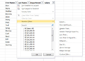
   

   Figure 7–19. Number filters

2. These are pretty easy, too. Clicking any of these options will again unfurl the Custom AutoFilter dialog box (except the Top 10... option, which will call up its own distinct dialog box), as shown in Figure 7–20.
   

   Figure 7–20. By the numbers: Just type a value and click OK.

3. This should be pretty self-evident by now. If you want to see all the staffers earning more than $30,000, just type 30000 and click OK.

You may also want to take special note of the Top 10… option, which lets you filter the top (or bottom) 10 values in the field—or the top 20, or the top 5, or any value you specify (see Figure 7–21).

Figure 7–21. The Top 10... option: Better than a Letterman list

Just click (or type) in the field exhibiting the default 10 and replace it with any other value, if you want to. And think big: imagine a set of test grades for a lecture class of 200 students, and think how simple would be to determine its top 10 highest scores. Also, if you click the drop-down arrow by Items field, you'll call up a Percent option, which lets you find out the top 10 percent of all scores instead.

Filtering Multiple Fields

In addition, you can filter the filter results. That means, for example, that starting with the result in which the Sales staff has been filtered, we could then execute a second filter—say, to find all the Sales personnel who earn more than $35,000. We'd do that by next clicking the Salary drop-down arrow and filtering for salaries above $35,000—using the number filters from the previous section. After that double filter is completed, only Ned Paulson would remain on the screen, because he's the only salesperson who earns over $35,000 (see Figure 7–22).

Figure 7–22. First we filter the Sales personnel, and then we filter those results by Salary.

Tables: Adding User-Friendliness to Your Database

Working with a database and adding records to it is generally a pretty easy task, but Excel provides the user with a way to make the process even easier—by transforming the database into a table. A table is a database to which some ease-of-use features have been added—features that spare the user from some of the drudgery associated with data entry (e.g., automatically copying a new formula to all the rows in the table). Let's turn our database into a table, and we'll see how it works:

1. Click anywhere in the database. Then click the Insert tab and select Table from the Tables button group. Doing so brings up the dialog box shown in Figure 7–23.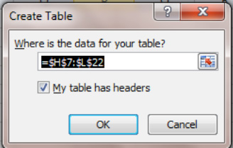
   

   Figure 7–23. Turning the tables on a database

2. Click OK, and then click anywhere in the worksheet to deselect the database. You'll see the results shown in Figure 7–24.

Figure 7–24. The database, now a table

You'll also see a Table Tools contextual tab, which we'll discuss shortly. The most obvious change produced by the table is the data's new format, in which the database records are colored alternately blue. These are called banded rows, an effect that makes the records easier to read. But there are features to a table that aren't quite so obvious, including these:

• The filter is turned on (although you can still turn it off in the standard way by clicking the Filter button).
• The header row in a table always remains on the screen. That means that if the table contains hundreds or even thousands of rows, and you scroll down the table, that first row will nevertheless stay in view. Take a look at the example shown in Figure 7–25.
  

  Figure 7–25. The header row's still on the screen—but look at the row numbers!

• The table receives a name—by default, Table1. (These names proceed in sequence; your second table will be called Table2, your third Table3, etc.) Whenever you click in the table, its name will appear in the Table Name field in the Properties button group on the Table ToolsDesign tab. You can also rename a table by clicking in the table and clicking in the Table Name field, typing a new name, and pressing Enter. The table name will appear when you click the drop-down arrow in the Name box; click the name and the table will be selected.
  

  Figure 7–26. A table renamed. Note the Name box.

• If you enter additional records (or rows) to the table, they too will automatically exhibit the same format.
• If you add a new field (or column) to the table, it too will display the new format.
• This one is important. If a field has formulas in it, any new records added to the table will automatically receive the formula, too (with the appropriate absolute or relative cell addressing figured in).

For example, suppose our pre-table database had a Raise field, in which every salary was awarded a boost of 5 percent (see Figure 7–27).

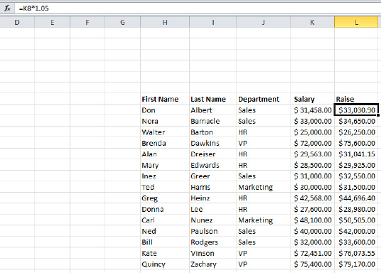
Figure 7–27. Pay day. Note the formula in the formula bar.

Once those raise formulas are in place and the database is then converted into a table, any new records you enter will also display the 5 percent raise, because the formula in the Raise field will write itself. Moreover, if you edit any one of the formulas in the Raise field, the table will rewrite all the formulas in the column correspondingly—a very cool feature.

There are a few other table features that are good to know. For one thing, it's easy to add columns to tables; and for another, when you click anywhere in the table, the Table Tools context tab is triggered (see Figure 7–28).

Figure 7–28. What you see when you click the Table Tools context tab. Note that the entire ribbon is now occupied with table options.

Note the Table Styles button group. Clicking its drop-down arrows reveals a collection of predesigned styles that you can apply to the table (see Figure 7–29).

Figure 7–29. Table styles: Just click one

You can inspect any of the table styles in preview mode by resting your mouse over it before you click. The table will exhibit the style.

To the left of Table Styles, you'll see the Table Style Options button group (see Figure 7–30).

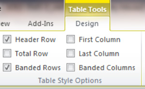
Figure 7–30. The Table Style Options button group

Its check boxes let you change specific elements of the table's appearance. If you uncheck Banded Rows and check Banded Columns, for example, you can realize the effect shown in Figure 7–31.

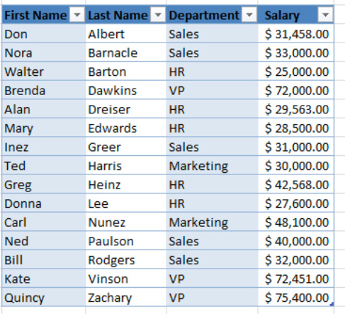
Figure 7–31. Banded table columns

And if you click the First Column and/or Last Column options, special effects (e.g., boldfaced text) will be imparted only to those columns, which you may want to emphasize.

The Table Style Options group also features an important Total Row selection. Click its check box and you'll see something like Figure 7–32.

Figure 7–32. The table, with a Total row appended at the bottom. If the total is too large to be seen, just widen the Salary column with autofit.

By default, the Total row adds the values in the rightmost field of the table, as shown in the figure. If that column contains textual data, the number of records is counted instead. And if you click in any other cell in the Total row, a drop-down arrow will appear, letting you select a mathematical operation for the data in that field (see Figure 7–33).

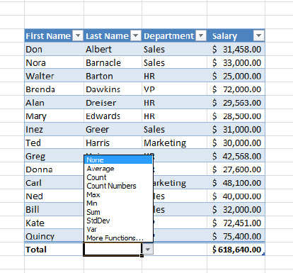
Figure 7–33. The Total row lets you perform a calculation on any field in the table.

What Excel is really doing here is enabling you to use one of its functions, which will calculate a result for the field in which you've clicked. Note the array of options made available; in Figure 7–33, in which we've clicked in a text field, we'll be able to tally a count of the number of last names in the table column. Click the down arrow by Salary and you can select a different calculation—say, an average. If you decide you need to add additional records to the table, you can click the Total Row check box a second time to remove it. You can then continue adding records.

Finding Duplicate Records in the Table (and Removing Them)

A classic data entry problem, one particularly besetting large databases, is the specter of duplicate records. It's not uncommon to discover the same names appearing repeatedly in large lists, and if you're the person charged with maintaining the database, you'll need to do something about it. Excel's tables are equipped with a Remove Duplicates feature, which speeds the task of winnowing those doubles from the data.

The first order of business in removing duplicates is deciding exactly what constitutes a duplicate. After all, Jane Walsh and John Walsh share a last name, but you're not likely to declare them duplicate entries. What you usually want to sift out are entire records that are identical—that is, two John Walshes—although it always isn't that simple. J. Walsh and John Walsh, both of whom record an address of 123 Broadway, might very well qualify as duplicates, too.

1. To see how Excel helps you with this task, pick out an empty area of the worksheet and enter the simple database shown in Figure 7–34. Remember that the size of the database is irrelevant. The Remove Duplicates options works the same way in every case.
   

   Figure 7–34. Double take: Searching for duplicates

2. Then convert the database to a table. Note that the “My table has headers” check box won't be checked, and that's because all the data in the database, including that in the top row, is text, so Excel can't tell if there's anything special or different about that top row. We thus need to tick the check box in order to let Excel know that we do want a header row.
3. Then click the Remove Duplicates button in the Tools button group, which will bring up the dialog shown in Figure 7–35.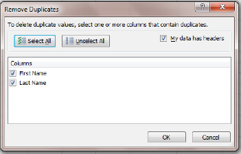
   

   Figure 7–35. The Remove Duplicates dialog box

4. You can probably figure out what to do next—just click OK. Because our table contains two people with the same last name but different first names, we leave both columns checked, which means that Excel will search the data only for records in which both fields are identical. When you click OK, you'll see the message shown in Figure 7–36.
   

   Figure 7–36. Yeah, “1 duplicate values” needs a grammar check . . . but it worked!

5. Click OK and you'll be left with three records, as one of the two John Walshes has been deleted.

Converting a Table to a Range

If you want convert a table back to the standard database with which you started, click Convert to Range in the Tools button group on the Table Tools tab. You'll be prompted to convert the table back to a “normal” range (as Excel puts it)—just click OK. Remember, after all, that a database is also just a range, too.

And given the advantages of turning a range into a table, why would you want to return it back to standard range status? That's a good and subtle question, and while you're not likely to convert it back to a normal range, there are some potential reasons why you might. For one, if you delete a record in a table—even the last record—the records on either side of the deleted row still remain in the table, and that means the blank rows will appear in pivot table reports.

Summary

Excel's sorting, filtering, and table features make the tasks of ordering and tracking down information from your data easy. But the techniques discussed so far may not answer all the questions you'd like to ask of your data. For example, what if you want to learn the average salary of your employees not across the whole company, but broken out by department? Or what if you need to know how much money each salesperson has earned per month? Or how much money you spend per month by budget category? Or perhaps you need to determine university students' grade point averages by their major. In the next chapter we're going to explore a powerful Excel feature that will help you with these questions and more: pivot tables.