7
Other Experimental Designs
Introduction
Over the years, the need to develop experimental designs that efficiently address important issues in the face of various constraints on experimental materials, protocols, and costs has led to the creation of new experimental designs. We have seen some examples:
- The shoe research manager needed to compare three tread designs in a situation where it was advantageous (for reasons of statistical precision) to use blocks (boys) that had only two experimental units (feet) in each block. Balanced incomplete block designs, developed for agricultural needs, provided a clever and efficient way to do that.
- Industrial processes posed new problems that agriculturally motivated designs did not address adequately. Industrial processes often involve a large number of process variables, in which case running an experiment with a full factorial set of treatment combinations is often prohibitive because of cost or time requirements. This constraint led to experiments with all factors at only two or three levels. Then, when there are enough factors that full factorial treatment combinations still become excessive, research led to the selection of cleverly selected fractions of the set of all possible factor combinations. There is no free lunch, though. We usually pay a cost for fractionalization in that the design then cannot detect interactions that might be important. If subject-matter context supports assuming certain interactions are negligible, this cost is often acceptable. If the experiment is a “screening” experiment, aimed at finding the most important factor effects as a preliminary to deeper experimentation with a subset of potential factors, this sort of staging can be an effective strategy. These sorts of trade-offs and decisions are made based on subject-matter knowledge and theory and helped by theory and analyses pertaining to statistical precision and the efficiency of candidate designs. It is not easy to make these decisions. They are not readily reduced to an algorithm.
Thus far in this text, we have considered two basic families of experimental designs: the completely randomized design and the randomized block design. In these designs, treatments are either assigned to a single set of experimental units completely at random, or they are randomly assigned to experimental units within each of multiple blocks of experimental units. Variations within these two families of designs have had to do with treatment or block structure. Both blocks and treatments can have multifactor structures, and both block and treatment factors can be either quantitative or qualitative. These aspects of the design affect the analysis, but do not change the basic structure of the design—the way treatments are assigned to experimental units. As broad as these two families are, extensions or modifications are still called for in many contexts. In this chapter, we consider some additional designs that modify or extend the basic CRD and RCB designs in various ways. Designs that depart from these basic structures are also discussed.
Latin Square Design
Example: Gasoline additives and car emissions
Reducing the emissions from automobiles is an area of ongoing widespread research. Federal and state governments set progressively lower limits, and regulators evaluate automobiles and fuels to determine whether limits are met or adequate progress is being made. Researchers therefore search for effective and cost-effective methods to reduce emissions. In Chapter 5 we saw an experiment pertaining to the effects of the ethanol/gasoline/air mix on CO emissions from automobiles. We now consider another emissions reduction example from Box, Hunter, and Hunter (2005). The following story is mine.
Suppose that a chemical manufacturer has developed three candidate gasoline additives. The director of research wants to do some testing to compare the additives. Preliminary tests on the company’s test engine have shown some apparent differences among the additives, but the director now wants a more stringent, realistic test. He wants to test these additives under the sorts of conditions that real drivers driving real cars in real traffic impose. He hires a testing lab to design and conduct an experiment.
After some fruitful discussion, the test lab rep says, “How about this: You provide us with four cars and we will instrument them”. You choose the cars to cover a reasonable variety of makes and sizes. They will be instrumented to capture and measure the emissions produced by a drive of whatever specified duration and driving conditions we decide on. I will employ just one driver in order to eliminate driver-to-driver variability and hold down costs. Driving each of the four cars, he will make one run using gasoline treated with each of the three additives plus a control run with no additive, in a random order with suitable purging of the fuel tank, fuel lines, carburetor, and exhaust pipes and chambers between runs. Thus, a total of 16 test drives. Showing off, he adds: “This is a randomized block experimental design with four blocks (the cars) and four treatments (the additives, counting the control condition of ‘no additive’ as one of the additives).”

The director replies, “I think drivers can make a difference. Two drivers driving the same car are apt to produce different amounts of emissions (from the engines, mind you) just because of driving style. I think we need more drivers in the experiment.”
The lab rep says, “OK, I’ll hire four different drivers. I’ll (randomly) assign each driver to one of the cars for the duration of the test. Each of the four car/driver combinations will make single runs using each of the four additives, in a random order, as before. Still a total of 16 test drives.”
DIRECTOR:
LAB REP:
DIRECTOR:
LAB REP:
A week later, the lab rep reports back. “That Latin thingy looks like a possible solution. Here’s a table (Table 7.1) that shows the combinations of cars, drivers, and additives we will run.” The experiment still has a total of 16 runs.
Table 7.1 4 × 4 Latin Square Design for Additive Experiment. a
| Driver | Car | |||
| A | B | C | D | |
| I | A1 | A2 | A4 | A3 |
| II | A4 | A3 | A1 | A2 |
| III | A2 | A4 | A3 | A1 |
| IV | A3 | A1 | A2 | A4 |
a Cell entries denote the additive assigned to a given car/driver combination.
“This table has a special characteristic: Each additive appears once in each row and each column. That is, each additive is run once with each car and each driver. Thus, when you compare the Additive means, each mean is calculated over runs that include all four cars and all four drivers. This balance means that we will get fairly clean comparisons of the effects of the four additives: the car and driver effects will cancel out. My own FLS, who happens to be my sister-in-law, says that the assumption we’re making is that the differences (in emissions) among additives should be consistent across cars and drivers and car/driver combinations. Similarly, we’re assuming that the difference between drivers should be consistent across cars; lead-footed in one car, lead-footed in the others.”
DIRECTOR:
They then work out the protocol. Each test drive is to follow a specified course of 150 miles, with a mix of urban and rural driving, at the posted speed limits, conditions permitting. Each driver’s four runs will be done in a random order. The engines, fuel tanks, and exhaust systems will be carefully purged between runs. At the end of each run, the cumulative emissions data will be collected, and perhaps, other variables such as elapsed time, fuel consumption, and ambient temperature will be collected and entered into an Excel spreadsheet. The test managers will also check the odometers to be sure the drive covered 150 miles.
Incidentally, as is often the case, there is a measurement issue in this experiment. You could measure emissions per mile driven or emissions per gallon of fuel consumed (or both). The former measures the combined effect of engine design and additive. The latter measures additive effect more directly.
The experiment was conducted without a hitch, and the emissions data (in coded units) are given in Table 7.2.
Table 7.2 Results of Car Emission Latin Square Experiment. a
Source: Reproduced from BHH (2005, Table 4.8, p. 157), with permission of John Wiley & Sons.
| Driver | Car | |||
| A | B | C | D | |
| I | A1 | CL | A2 | A3 |
| 19 | 24 | 23 | 26 | |
| II | A2 | A3 | A1 | CL |
| 23 | 24 | 19 | 30 | |
| III | CL | A2 | A3 | A1 |
| 15 | 14 | 16 | 16 | |
| IV | A3 | A1 | CL | A2 |
| 19 | 18 | 19 | 16 | |
a Emissions as a function of car, driver, and additive.
Details
Randomization in a Latin square design is done by starting with a basic Latin square and then randomly assigning the factor levels to the symbols. In this experiment, when the additives were randomly assigned to symbols, the treatment of no additives was labeled A2 in Table 7.1. This treatment is denoted by CL, for control, in Table 7.2. Also, the random assignment of the three additives to symbols resulted in A4 being assigned the A2 additive; A1 and A3 actually were assigned the A1 and A3 symbols. The additive labels in each cell of Table 7.2 are the chemical company’s additive names, not the generic names in Table 7.1. I point all this out in case any alert reader wonders why the A2s in Table 7.1 are not in the same boxes as they are in Table 7.2.
(All this detail is part of my story creation. The original example in BHH did not identify one of the additive levels as the control condition (no additive), but that seems to me the right thing to do in an experiment like this. While we want to know whether any additive enables car manufacturers to meet regulatory limits, we also want to know how much reduction it provides compared to adding nothing. That knowledge could help define further research.)
Let’s look at the Latin square design in the contexts we have seen in previous chapters. First, note that the Latin square design could be called a very incomplete block design. In this example, we have 16 blocks, the car/driver combinations, with only one experimental unit (a 150 mile prescribed drive) per block. It’s going to be difficult (impossible) to measure the variability among experimental units or variability among treatment differences within a block in this situation (as with the boys’ shoes). All of our information about additive differences comes from interblock comparisons; there is no intrablock information.
In the Latin square, each additive is assigned to four blocks but, systematically, not at random. That is why the Latin square design is not a special case of the randomized block design. The assignment is constrained to achieve the balance discussed earlier. Randomization enters the design as described previously in this section by randomly assigning the A, B, C, and D labels to the four cars in the experiment and by similarly randomly assigning the labels for drivers and additives. Also, when order might be a concern, as here, the 16 runs should be done in a random order. If they don’t have a schedule laid out, and a test manager to assure the schedule is followed, test personnel might be tempted to run a more convenient order. For example, all four drivers might do their A1-additive runs on Monday, their A2-additive runs on Tuesday, etc. That reduces the chance of putting the wrong additive in a car on any given day. But, it’s possible that there could be a learning curve or a boredom trend at work in this test, so a finding of apparent differences among additives could be really the effect of learning or boredom in repeatedly driving the 150 mile course.
Second, note that the Latin square is a fractional factorial arrangement of blocks and treatments. The emissions experiment has three four-level factors (two block factors, one treatment factor). One replication of the full set of factorial combinations (the alternative design that was rejected as too expensive) would have 4 × 4 × 4 = 64 runs. The 4 × 4 Latin square design specifies a particular 1/4 fraction of those 64 runs.
Analysis 1: Plot the data
I have repeatedly said that initial data plots should show all the dimensions of the data, if possible. The fractional nature of this experiment makes it impossible to produce a meaningful data display showing all four dimensions of the Latin square design: cars, drivers, additives, and emissions. For example, if you plot emissions versus additive, by car, the four points for a given car differ not only by additive but also by driver, so you cannot graphically isolate the effects of car, driver, and additive. This is the graphical manifestation of the fact, as will be seen, that by the fractional nature of this design, one cannot evaluate interactions in the ANOVA.
Under the assumption of no interaction, we can (and in this case, have to) go straight to main-effect plots, which are given in Figure 7.1. Each point in Figure 7.1 is the average for a given factor level, averaged over the four runs in the experiment that were done at that factor level. For example, the four runs, for additive A1, included all four cars and all four drivers as specified in the Latin square design table. All three plots have the same vertical axis for ease of comparison.

Figure 7.1 Average Emissions by Car, Driver, and Additive.
Figure 7.1 shows, by the greater spread among the four drivers, that drivers apparently have more of an effect on car emissions than do cars (which might be an indication that emissions were measured on a per-gallon-consumed basis, not a per-mile-driven basis) or additives. Additive was a qualitative treatment factor, as far as we know, so the apparent linear trend for additives in the figure is not meaningful. It is just happenstance in the random assignment of labels to additives. Now, if we found out that A1–A3 were three decreasing concentration levels of one additive (and CL was zero additive), then additive is in fact a quantitative factor, and we would want to plot the emission averages versus concentration to see if increasing concentrations resulted in reduced emissions. What the additive main-plot display shows is that all three additives resulted in lower emissions than the control treatment of no additive. That’s an encouraging sign. We will soon see if that apparent difference is “real or random.”
First, though, if there are no, or only minor, differences among cars, then it makes sense to plot the data in a way that ignores cars. One of the nice features of the Latin square (and other well-chosen fractional factorials) is that if one of the three factors in the experiment turns out to have a negligible effect, the design collapses to a balanced two-factor design. By ignoring cars, we’re left with a 4 × 4 arrangement of drivers (blocks) and additives (treatments) in what is a randomized block design with one replication of each treatment in each block. Thus, we display the data in an interaction plot. Figure 7.2 provides that interaction plot of emissions versus driver.

Figure 7.2 Interaction Plot of Emissions Data by Additive and Driver.
Figure 7.2 shows an intriguing pattern. The lower-left panel shows that for drivers I and II (the red and black plotting symbols), there was a substantial difference in emissions for the four additives, while for drivers III and IV (green and blue), there was not. This looks like a classic case of interaction, but with no replication, we have to treat these inconsistencies as random variation. Further experimentation is necessary to resolve the issue of real versus random interaction. Based on these data, I would like to have an off-the-record chat with these drivers to see if they deviated from the assigned drive in any way. If a driver drove over the speed limit and then took a half-hour break midway through the run for lunch or other refreshment, that might affect his car’s emissions. Not accusin,’ just sayin.’
From the graphical evidence, we might choose A1 as the winning additive: it had the lowest emissions for two drivers and not so bad for the other two drivers. On the other hand, if we could get everybody to drive like drivers III and IV (the green and blue symbols), we might be able to get away with using no additive. Obviously, though, we need a lot more data before making any such decisions that have nationwide ramifications. Some possible follow-on experiments are discussed in a later section.
ANOVA
The ANOVA for this Latin square experiment can separate out the variation associated with the main effects of car, driver, and additive. No interactions can be evaluated. The MSs for all three ANOVA entries are calculated from the variances of the four means in each of the panels in Figure 7.1. The ANOVA for the emissions data (Table 7.3) shows that only the differences among drivers stand out appreciably above the residual error variability. This result is consistent with the visual impression in Figure 7.1. The aforementioned data plots have shown us the inconsistencies that contribute to this error variability.
Table 7.3 ANOVA for Emissions Experiment.
| Source | DF | SS | MS | F | P |
| Car | 3 | 24 | 8.0 | 1.5 | .31 |
| Driver | 3 | 216 | 72.0 | 13.5 | .004 |
| Additive | 3 | 40 | 13.3 | 2.5 | .16 |
| Error | 6 | 32 | 5.3 | ||
| Total | 15 | 312 |
Just as we simplified plots of the data by ignoring cars, we can simplify the ANOVA by dropping the car source of variability (which means merging these three df and corresponding SS with the error line in the ANOVA). (Mathematically, we’re taking the car effect out of the statistical model underlying the analysis.) The result, in Table 7.4, doesn’t change our conclusions: substantial differences among drivers, some evidence of differences on average among additives, but no way to test for interaction. We need a bigger and better experiment to decide if we need better additives or better drivers in order to reduce automobile emissions.
Table 7.4 Reduced ANOVA of Emissions Data.
| Source | DF | SS | MS | F | P |
| Driver | 3 | 216 | 72.0 | 11.6 | .002 |
| Additive | 3 | 40 | 13.3 | 2.14 | .17 |
| Error | 9 | 56 | 6.2 | ||
| Total | 15 | 312 |
Discussion
This example illustrates a larger truth: findings in a tightly controlled laboratory experiment may not carry over to a much noisier environment, especially one involving people who have a myriad of unpredictable ways to use and abuse the scientist’s or engineer’s creations. Variability happens! Anybody who makes or sells consumer products knows this. We saw this phenomenon manifested in the case study in Chapter 1 and in the textile production example in Chapter 6. Machines were consistent; human operators were not (because of human nature, not deliberate actions). One thing though, the results of this experiment validated the research director’s aversion to running the experiment with one driver only. It also validated his recognition that the additives needed to be evaluated in realistic driving situations, not just in the lab. His company would like eventually to market their additive to millions of drivers. Betting the company’s bottom line on only lab data, or on one driver’s data, is not an acceptable risk. Inadequate market research has torpedoed more than one product. Remember New Coke? Remember the Edsel? (Well, probably not.)
Follow-on experiments
There are various ways to extend this emissions experiment. These include:
- Repeat the exact same Latin square experiment: same drivers, cars, and additives, same test and measurement protocols. This would provide a direct measure of repeatability—variability.
- Run the same Latin square again but with four different drivers.
- Run a different Latin square, by rerandomizing the assignments of factor levels, with the same drivers, cars, and additives. Choose the second Latin square so that the combined set of 32 runs will help one separate out some of the interactions. (The combinatorial problems that can be worked in this situation are beyond the scope of this text.)
- Run a different Latin square with four new drivers, same four cars and additives.
- Run the 48 runs needed to complete the full 43 combinations of drivers, cars, and additives. The design can be analyzed as a complete three-way classification. Note, though, that this two-stage design (and randomizations) is not the same as a RBD with 16 blocks, four treatments assigned randomly to four experimental units in each block. The analysis would need to reflect the staging of the experiment which, in effect, is an additional blocking factor.
Here, the additive manufacturer is considering augmenting the first Latin square with another Latin square to help resolve some of the questions raised by the first experiment. The lapse in time between the two experiments could introduce some new sources of variation. The drivers might say, “You mean you want me to take four more drives over the same course? Boring.” (The test director might want an observer to ride with each driver to assure protocol is followed and to collect ancillary data—for example, traffic conditions.) In hindsight, it might have been good to consider the alternative of a replicated Latin square design (total of 32 runs) which would fall between the 16-run Latin square and the 64-run randomized block.
Some of these replicated Latin square designs are used in the context of “repeated measures” designs discussed later in this chapter. In these designs, individual experimental units are measured repeatedly. They may also have different treatments applied to them sequentially.
Exercise
Write out the ANOVA tables, Source, and df, for alternative designs 1, 2, and 5 in the above list.
Extensions
The emission example had two blocking factors and one treatment factor. Other experimental situations may have one blocking factor and two treatment factors. This turns the design into an incomplete block design. For the 4 × 4 Latin square, we would have four blocks of four experimental units and 16 treatments. The Latin square layout would define which four treatment combinations are assigned to each block, and those four combinations would be randomly assigned to the four experimental units (runs, in this case) in a block.
Latin squares of any size can be constructed. Cochran and Cox (1957) catalog some designs up to 12 × 12. Not all physical situations lend themselves to having three factors with the same number of levels. However, there are some tricks to pull. For example, in the emissions situation, another candidate design could have been a 5 × 5 Latin square with five cars and five drivers. The treatments could have been the three additives and two control runs.
In the basic Latin square design, the three factors are generically called rows, columns, and treatments. It is possible that any of these three generic factors could be factorial combinations of other factors. For example, a 6 × 6 Latin square might be run in which the six treatments were the six combinations of a three-level and a two-level factor. Then, the 5 df for treatments in the ANOVA could be separated into, say, factor F1 with 2 df, factor F2 with 1 df, and F1 × F2 interaction with 2 df.
Another extension is to add a fourth factor. If the Latin square is of at least dimension 3 × 3, this can be done in a balanced way. This four-factor design is called—are you ready?—a Graeco-Latin square. Table 7.5 gives a 4 × 4 Graeco-Latin square design.
Table 7.5 4 × 4 Graeco-Latin Design.
| Row | Column | |||
| A1 | B3 | C4 | D2 | |
| B2 | A4 | D3 | C1 | |
| C3 | D1 | A2 | B4 | |
| D4 | C2 | B1 | A3 | |
The alphanumeric characters in the table indicate the combinations of treatment factors to be run in each row/column combination. For example, the upper left entry of A1 means that, say, when driver 1 uses car 1, the treatment combination will be factor1 at the A level and factor2 at the “1” level. Note that each number occurs once in each row and column and once with each letter. This balance means that in the ANOVA, we can separate the SS into rows, columns, Factor1, and Factor2, each with three df. This leaves 3 df for error. Under the (strong) assumption of no interactions among the blocking and treatment factors, this experiment provides clean estimates of the effects of all four factors.
In fractional factorial terminology, the 4 × 4 Graeco-Latin square is a 1/16th fraction of a 44 set of factor combinations.
In the Table 7.5 design, the second treatment factor could be the order of the runs. In the preceding, the Latin square experiment was done by randomizing the order each driver did his four runs. Alternatively, we could balance the run orders using this Graeco-Latin square. Thus, driver 1’s first run would be car (column) 1 using additive A. Her second run would be car 4 using additive D, then car 2 with B, and then car 3 with C.
Latin square and Graeco-Latin square designs offer a chance to evaluate the effects of three or four factors with a minimum of runs. They yield clean estimates of the effects of these factors only if there are no interactions among any of them, as is the case with fractional factorial arrangements in any situation. However, as is stated in BHH (2005, p. 160), to use a Latin square design to study process factors known to interact is an “abuse” of the design. Subject-matter knowledge is required to avoid this abuse and the resulting misleading conclusions.
Split-Unit Designs
Consider again the commercial-scale tomato fertilizer experiments discussed in Chapter 3. Suppose it was decided to run the experiment with 300 plants treated with Fertilizer A and 300 plants treated with Fertilizer C. Rather than randomly assign fertilizers to individual plants, suppose it was decided that the experimental unit would be a plot with 30 plants (perhaps a 6 × 5 grid, perhaps a row). Fertilizers would be applied simultaneously to these groups of contiguous plants, which is much more convenient than applying fertilizer one plant at a time. Now, the experiment would have a total of 20 experimental units (consisting of 30 contiguous plants), and each fertilizer would be randomly assigned to 10 of these eus.
Suppose that the experimenter decides that the amount of fertilizer is another important factor. If the experiment is done with just one level of fertilizer and we see a difference between Fertilizers A and C, could it be that the same difference would occur if we had used either a higher or lower amount of fertilizer? Also, will applying more fertilizer lead to more tomatoes? If so, will increased yield offset the increased expense? I don’t want to wait until the next crop and run experiments at a different level of fertilizer. Can we vary the amount of fertilizer in the current design? In particular, could we consider three levels of fertilizer, say, low, medium, and high? Inquiring (scientific) minds want to know. The tomato mogul asks his FLS, “How can we include fertilizer amount in the experiment?”
The experiment now has six treatments: the six combinations of two fertilizers each at three levels. The FLS comes up with two experimental designs.
Let’s suppose we start over and redefine the experimental unit structure as groups of 10 plants. Our layout would then have 60 eus. With each fertilizer at three amounts, this makes a total of six treatments. We would then randomly assign each of these six fertilizer/amount combinations to 10 eus each. This would be a completely randomized experiment with six treatments in a 2 × 3 structure with 10 replicates (of groups of 10 plants) of each.
On the other hand, suppose we split each eu of 30 plants that have already been randomly assigned a fertilizer into three subunits of 10 contiguous plants each. Within each experimental unit, then, we would randomly assign the three fertilizer levels to one subunit each. This way, we could measure the effect of fertilizer level within each experimental unit (contiguous group of 30 plants). The variability among the three subunits within an experimental unit should be less than the variability among the experimental units over the whole field. Thus, we ought to be able to estimate the effect of fertilizer level more precisely than with the completely randomized experiment.
In this second experimental design, the design at the subunit level is a randomized block design. Each “main-plot” unit (30 plants) is a block of three “subplot” units, randomly assigned the three levels of the fertilizer assigned to the main plot. We started with a completely randomized design for the fertilizer factor and then, in essence, embedded a randomized block design for the level factor. This gives us an experiment with two sizes of experimental units and with two levels of randomization. Figure 7.3 illustrates the experimental structure and randomization. It shows a subset of the main units and their fertilizer assignment; then within each main unit, the three subunits are shown with their randomly assigned levels of fertilizer.

Figure 7.3 Schematic Illustrating Split-Unit Design for Tomato Fertilizer Experiment. The design has 20 main-plot units, with each fertilizer randomly assigned to 10 units. Each main-plot unit is divided into three subplots, and the three fertilizer levels are randomly assigned to one subplot unit each.
This hybrid design is called a split-unit or split-plot design. The latter term reflects the design’s origins in agricultural experiments such as the tomato fertilizer experiment, where plots of land are split into subplots. Split unit is a more general term: one experimental unit is split into subunits to which subsequent treatments are applied. Manufacturing processes often involve a number of sequential steps, and such situations make split-unit experimental designs feasible and practical. At selected steps, the material being processed can be split into subbatches for the application of factors involved in the next step.
Split-unit experiments can be difficult to recognize. A spreadsheet of data can look like any of a variety of multifactor experiments. It can take a lot of detective work to find out what factors, if any, are blocking factors and which are treatment factors and, critically, what were the experimental units for the application of the treatment factors. You have to understand the experimental protocol before you can make sense of the data and extract any message hidden in that cloud (see front cover). The following example is a case of aggregated units, rather than split units. One treatment factor is applied to individual units; then subgroups of units are aggregated for the application of the second treatment factor. So, the experiment has treatment factors that are applied to different sizes of experimental units via aggregation, rather than splitting. Recognizing this is key to running the correct ANOVA.
Example: Corrosion Resistance
I again turn to the classic Box, Hunter, and Hunter (2005) text for an example. As always, the following story is my own embellishment.

A team of chemists in a chemical products company is charged with developing coating materials that will prevent corrosion on structures such as buildings and bridges made of steel. Protection from corrosion is important to assure structural integrity and to minimize the amount of inspection and maintenance that is required.
Coating is applied to steel parts by spraying the coating on a part and then curing (baking) the part at a specified temperature for a specified time. At this stage of their investigation, the chemists have selected four coating materials to compare. They have settled on what the curing time should be, but they want their experiment to include curing temperature as an experimental variable to be investigated. The reason for this objective is that an ideal coating material should provide good corrosion prevention over a range of curing temperatures. This is an important characteristic because steel companies and other customers for their coatings will not necessarily be able to control curing temperature very precisely and consistently. A coating that is effective when cured at 370° (F), say, but ineffective if cured at 360° or 380° is not a good product, particularly if the user’s furnace cannot control temperature that precisely. The terminology sometimes used is to say that such a coating is not “robust.” Robust products mean better structures, happier customers, and more sales. That’s the ultimate goal. More discussion of robust designs is given later in this chapter.
Developing and improving chemical products is a statistics-rich environment. Efficient experimentation is essential to success. Thus, large, successful chemical companies have in-house departments of friendly, local statisticians. Smaller companies often hire university or private statistical consultants, which is the case here.
Two chemists meet with a statistician from the local university. They describe the coating and curing processes and tell the statistician that they have 24 steel bars to use in the experiment. They say that after a bar is coated and cured, it is subjected to a corrosive environment, and then corrosion resistance is measured by standard techniques.
After some discussion, it is decided to experiment at three temperatures, 360, 370, and 380°F, for reasons discussed earlier. The statistician suggests that they run all 12 treatment combinations, four materials at three temperatures, on two bars each. The treatment combinations will be randomly assigned to bars and run in a random order. Thus, the design would be a completely randomized experiment with 12 treatments applied independently to two randomly selected experimental units each. The FLS even goes so far as to lay out the random treatment assignment and a random order of experimentation. He also stresses the importance of true replication: between each run, the coating and curing processes must be shut down and restarted in order to really have multiple independent applications of treatments to experimental units.
The chemists frown. “It takes a lot of time to shut down the temperature chamber and restart it. Besides, our chamber will hold more than a single bar. If we cure several bars at a time, we’ll save a lot of time and expense.” They suggest putting two bars with each coating in the chamber for a given temperature setting. Thus, they could do eight bars at 360°F, say, as one “heat,” and another eight at 370°F and the remaining eight at 380 F. Coatings would be randomly assigned to bars within each heat group. That way, the experiment could be done in three heats, rather than 24. “Neat, huh?”
“I’m sorry,” says the FLS (searching for a polite way to say that this is a bad idea). “With only one heat at each of the three temperatures, your experiment won’t have any replication of the curing-temperature treatment. We won’t be able to estimate the inherent variability of the process and won’t be able to tell whether any apparent differences among temperatures are real or random.”
“I have an idea, though,” he says. “How about if we do heats of four bars—one with each coating material. This will mean a total of six heats, two at each temperature, thus (minimally) replicating the temperature treatment. We should randomly assign temperatures to groups of four bars and randomly order these six heats. We also should randomize the oven positions for the four bars in each heat. How about this as a workable compromise?”
“Well, OK,” say the chemists. “But could we run the heats in this order: 360, 370, 380, 380, 370, 360? Ramping up and then ramping back down will save us time.”
The FLS is not too happy with this plan, but he doesn’t want to push too hard. He asks, “In your experience is there any carry-over effect, or hysteresis, when you do this?” “No, don’t think so,” respond the chemists. So, that is the way the experiment is run.
Note that this experiment has treatments applied to two different experimental units. It is not a completely randomized design. Coating materials are assigned to single bars with six bars being randomly assigned to each of the four coatings. Thus, for the coating treatment, the design is a CRD, and a single bar is the experimental unit that gets the randomly assigned coating material. However, the curing-temperature treatment is applied to groups of four bars; thus, the group of four bars is the experimental unit for the temperature treatment. We therefore have a split-unit design, in reverse. We got this experimental structure by aggregating subunit experimental units (the coated bars), rather than splitting main units, as in the aforementioned agricultural example. The result is the same, though: different experimental units for different treatment factors in the same experiment. Our analysis will have to reflect that experimental structure.
Table 7.6 Corrosion-Resistance Experiment Data.
Reproduced from BHH (2005, Table 9.1, p. 336), with permission of John Wiley and Sons.
| Temp. (°F) | Heat | Coating | |||
| 1 | 2 | 3 | 4 | ||
| 360 | 1 | 67 | 73 | 83 | 89 |
| 6 | 33 | 8 | 46 | 54 | |
| 370 | 2 | 65 | 91 | 87 | 86 |
| 5 | 140 | 142 | 121 | 150 | |
| 380 | 3 | 155 | 127 | 147 | 212 |
| 4 | 108 | 100 | 90 | 153 | |
Analysis 1: Plot the data
Figure 7.4 gives a plot of the corrosion-resistance measurements versus the order of the heats, by coating material. The temperatures are also shown, ordered in the sequence in which they were done, as discussed. All 24 data points are shown in Figure 7.4, and each point is identified by its coating, curing temperature, and heat order. Thus, all dimensions of the data are captured in the plot.

Figure 7.4 Corrosion Resistance Plotted as a Function of Heat, Curing Temperature, and Coating.
Figure 7.4 exhibits some erratic behavior. The two 360°F heats, heats 1 and 6, differ substantially, as do the pairs of heats at 370 and 380°F. There is little difference between heats 1 and 2, run at 360 and 370°, respectively, while on the ramp down, there is a large difference between these two temperatures in heats 5 and 6. The data look like the chemists might not have been able to control the heat chamber temperature closely enough to be sure that they were getting reliable results. For example, consider heats 4 and 5. The lower temperature (370) yielded better resistance than the higher temperature (380) (subject-matter knowledge says that this should not happen). For heats 2 and 3, at the same pair of treatments, the order is reversed. If there is a temperature control problem in the experiment, this is embarrassing because the chemists picked the temperatures because of their concern that their customers may not be able to control temperature closely enough to get consistently good corrosion resistance. Or, maybe some data were mislabeled. The pattern would make more sense if heats 4 and 5 data were interchanged. It’s all a little disturbing, but, unfortunately, we cannot go to the source and pursue these questions.
The picture with respect to coatings looks more informative. Coating 4 is fairly consistently the best—the highest or near-highest corrosion resistance in each heat, especially the two 380°F heats.
To show the relationship of corrosion resistance to temperature, Figure 7.5 gives scatter plots of those two variables for each coating separately. The data points are labeled by the heat number to show how the bars are grouped in heats.

Figure 7.5 Plot of Corrosion Resistance versus Curing Temperature by Coating.
Figure 7.5 shows that there is some improvement of corrosion resistance as temperature is increased, but the pattern is different for the four coatings. This evidence of coating by temperature interaction is more clearly seen in an interaction plot (Fig. 7.6).

Figure 7.6 Interaction Plot of Corrosion Resistance Averages versus Temperature by Coating.
In Figure 7.6, each plotting point is the average corrosion resistance over the two heats run at the selected temperature. This figure shows that Coating 4 has markedly better corrosion resistance when cured at 380°F than do the other three coatings which have corrosion resistances that level off between 370 and 380°F.
ANOVA
Now, let’s construct the ANOVA for this experiment. At the main-unit level, the experimental unit is a “heat,” which is a group of four bars, all simultaneously cured at one temperature. There are six such main units; two for each of the three temperatures. Thus, at this level, the experiment is a completely randomized design with three treatments and two replicates for each. This part of the ANOVA therefore has the following structure.
Main-Unit ANOVA.
| Source | df |
| Temperature | 2 |
| Error1 | 3 |
The ANOVA entry labeled Error1 is pure main-unit experimental error: it is the variability between the two heats at each temperature, pooled across the three temperatures. I use the label, Error1, to distinguish this level of experimental variability from the subunit variability: next.
The subunit in this experiment is a single bar, and there are four in each main-unit group of bars (a heat). Each of the bars in each heat was randomly assigned one of the four coating materials. Thus, for the subunit part of the experiment, the design is a randomized block design with six blocks (the heats) of four experimental units (individual bars), and as is the case for a randomized block design, each of these subunits is randomly assigned one of the four coating materials. Each coating is applied to one bar in each “block.” Thus, the subunit ANOVA has the structure of a randomized block design with six blocks, four treatments, and only one replicate of each treatment in a block, as follows.
Subunit ANOVA.
| Source | df |
| Heats | 5 |
| Coatings | 3 |
| Error2 | 15 |
There is overlap between these two ANOVAs. The 5 df for heats in the subunit ANOVA are the same 5 df in the main-unit ANOVA, separated there into temperature (2 df) and heats within temperatures (3 df), which is Error1. Error in the subunit ANOVA is the heat by coating interaction—the variability of coating differences from heat to heat. That error needs to be further separated.
The error in the subunit ANOVA can be further resolved because of the structure of the heats: three temperatures, two main units for each. That is, the six heats were not nominally identical runs as was the case in Chapter 6 for the batches of material used in the penicillin production experiment. Part of the heat by coating interaction is actually the temperature by coating interaction, with 6 df (of error’s 15 df). The remaining 9 df consists of heat by coating interaction (3 df ) within each temperature. (In each temperature, there are two heats crossed with four coatings. Thus, there are (2 − 1) × (4 − 1) = 3 df for interaction.) Pooling these interactions across the three temperatures makes up the 9 df. This entry is labeled Error2, the subunit residual error. The full ANOVA has the structure shown in Table 7.7.
Table 7.7 ANOVA Structure for Corrosion-Resistance Experiment.
| Source | df | Main unit |
| Temp | 2 | |
| Error1 | 3 | |
| ------------------- | ------ | ------------ |
| Coating | 3 | Subunit |
| Temp × Coating | 6 | |
| Error2 | 9 | |
| Total | 23 |
The full ANOVA for the corrosion-resistance data is given in Table 7.8. Some statistical software is capable of separating the main unit and subunit ANOVAs, particularly the two error terms. Note the difference in the two error mean squares. Alternatively, one can run a one-way ANOVA for the temperature and heats within temperature and a two-way ANOVA on temperature and coating to get the entries in the Table 7.8 ANOVA. Error1 is the variability among heats (groups of four bars). Error2 is the variability among bars within the same heat.
Table 7.8 ANOVA for Corrosion-Resistance Split-Unit Experiment.
| Source | DF | SS | MS | F | P |
| Temp | 2 | 26 519 | 13 260 | 2.8 | .21 |
| Error1 | 3 | 14 440 | 4813 | 38.7 | .00 |
| -------------------------------------------------------------------------------------------------------------------- | |||||
| Coating | 3 | 4289 | 1430 | 11.5 | .002 |
| Temp*coating | 6 | 3270 | 545 | 4.4 | .024 |
| Error2 | 9 | 1121 | 125 | ||
| Total | 23 | 49 639 | |||
Often, it is the case that main-unit variability is larger than subunit variability. The two error MSs for these data have this relationship: Error1 MS is about 40 times the Error2 MS. This reflects the patterns seen in Figure 7.7. The connected lines for each coating are roughly parallel (small interaction), while the two heats within each temperature differ substantially.

Figure 7.7 Plot of Pulse Rate versus Time (min) by Subject and Drug.
Interpretation of the ANOVA starts with the F-ratio and P-value for the temperature by coating interaction. The small P-value reflects the pattern in Figure 7.6 in which the Coating 4 increase in corrosion resistance at 380°F differs from the other three coatings. The ANOVA confirms (as it should) the visual impression in Figure 7.6. If maximizing corrosion resistance is the objective, subsequent analyses such as confidence and prediction intervals would focus on Coating 4 and its temperature dependence. The producer of Coating 4 would instruct users to cure the coating at 380°F. However, this experiment started with the objective of finding a coating that delivered adequate corrosion resistance across the whole temperature range. Such “robustness” would enable a customer to produce corrosion-resistant steel even if they were not able to control temperature accurately within the 360–380°F range considered in the experiment. To address this issue, we need a definition of what minimum corrosion resistance is considered necessary. I won’t make up that part of the story.
My data-snooping habits would lead me to look deeper into why there is so much variability between the two heats run at each temperature. Could the assigned temperatures have been missed or the data mislabeled? For example, if heats 4 and 5 were reversed, the pattern in Figure 7.4 would be more like what I would expect, at least for the 370–380–380–370 middle four heats. The dismal performance of heat 6 at 360°F for all four coatings makes me wonder if the actual temperature was 360°F or if the curing time was not run as prescribed. Sometimes experiments raise more questions than they resolve. That’s why the sainted Sir Ronald A. Fisher (1938) stated,
To consult the statistician after an experiment is finished is often merely to ask him to conduct a post mortem examination. He can perhaps say what the experiment died of.
The post mortem continues—there are two other aspects of this experiment that might be at least partially responsible for the unusual variability seen in the experiment:
- The four coatings are actually defined by two other factors, B, the base treatment, and F, the finish, each at two levels.
- The four bars were randomly assigned to four positions in the furnace (see Table 9.1 in BHH) (2005, p. 336).
The two-factor structure of the coatings means that the three df for coating in the ANOVA can be separated into the ANOVA entries of B, F, and B × F, each with 1 df. When this is done (it is shown in BHH), the interaction is quite significant, meaning that the four coatings can be treated as four distinct coatings, as I have done. There are no consistent B or F effects to explain the coating differences.
Additionally, the T × C interaction in the ANOVA can be separated into B × C, F × C, and B × F × C, each with 2 df. In this case, only the B × F × C interaction is significant. High-order interactions are a sign of erratic patterns in the data.
The random, and hence unbalanced, assignment of bars to positions could also be a contributor to the variation in the data. I will leave it to the intrepid instructor or student to investigate this aspect of the data. The position and coating assignments are in Table 9.1a on p. 336 of BHH (2005). Another potential assignment is to redesign the experiment so that a possible position effect could be evaluated and balanced so that the coating effects could be more cleanly estimated.
Discussion
As stated prior to this example, it is often difficult to recognize split-unit designs after the fact. You certainly cannot detect splitting and grouping from a data table. Those who plan and conduct the experiment and know where experimental units were split or merged along the way may not appreciate the effect these actions have on the subsequent statistical analysis. When the data are dropped on the FLS’s desk, the full story may not be told. I have spent a lot of time asking experimenters polite questions, trying to reconstruct the scene of the crime, so to speak. Presented with the data organized as in Table 7.6, I would ask what this heat variable is and perhaps soon find out that the four bars in each heat were cured simultaneously, while coatings were applied to individual bars. If heat had not been shown in the table, I would probably note that there were consistent differences between the groups of four bars in each temperature and wonder if the experimenters had just arranged the data that way or if these differences reflected something about how the experiment was conducted.
Now, let us suppose (erroneously!) that the FLS asked to analyze the data looked at the table of data and said, “That looks like a completely randomized design with 12 treatments, consisting of combinations of four coatings and three temperatures and two experimental units in each treatment combination” (kind of like the poison/antidote experiment in Chapter 5). Therefore, the ANOVA is that of a two-way classification with two replications. Then the ANOVA would be that as shown in Table 7.9.
Table 7.9 Incorrect ANOVA of Corrosion-Resistance Experiment: Split-Unit Design Structure Not Recognized.
| Source | DF | SS | MS | F | P |
| Temp | 2 | 6519 | 3260 | 10.2 | .003 |
| Coating | 3 | 4289 | 1430 | 1.10 | .39 |
| Interaction | 6 | 3270 | 545 | .42 | .85 |
| Error | 12 | 15 561 | 1297 | ||
| Total | 23 | 49 639 |
This ANOVA merges the whole-unit error and subunit error that were properly separated in the split-unit ANOVA in Table 7.8. The whole-unit oranges are mixed with the sub-unit grapes into a bad-tasting fruit salad. Taking the analysis at face value, one would conclude that there is no temperature by coating interaction (i.e., the coating differences are consistent across temperatures—relative to the experimental error—and no overall differences among coatings). wrong! Temperature, as we have seen in our careful and correct analysis, has a strong effect on corrosion resistance, particularly for Coating Material 4. The conclusions drawn from the incorrect analysis are just the opposite (!) of the conclusions drawn from the correct split-unit ANOVA: no difference among temperatures and coating differences that are not consistent across temperature. (Jones and Nachtsheim (2009) also contrast the correct and incorrect analyses of this experiment and provide much more information on split-plot or split-unit designs.)
The morals of this story:
- Design matters.
- I’ll say it again: you can’t tell how an experiment was conducted just by looking at a data table.
Split-unit designs can be used in settings other than agricultural or industrial. For example, education researchers might evaluate teaching materials and testing methods as follows: first, some number of classes (defined, e.g., by location, grade level, and teacher) would be selected for the experiment. These might be chosen to be reasonably homogeneous, or they might be selected to span some range of demographic characteristics, depending on context and issues that the experimenters want to consider. The different teaching materials under consideration would be assigned to classes, either completely at random or randomly within demographic or geographic blocks. At the end of the instructional period, each class would be randomly divided into subgroups of students, and then the testing methods would be randomly assigned to these subgroups. (This assignment should be controlled by the experimenters. If test-method assignment is left to individual teachers, some bias could creep in—well-meaning teacher: “I think Susie will do best if she is tested by Method B.”)
Thus, in this experiment, for the treatment factor of teaching material, the experimental unit is a class. For the treatment factor of testing method, the experimental unit is a subgroup within a class. Conceptually, this is the same as the tomato grower’s experiment with fertilizer types and amounts discussed earlier in this section. (“The nice thing about statistics is that the nouns may change, but the verbs stay the same,” said Prof. Carl Marshall ( Oklahoma State University, ca. 1965).)
Additionally, in this experiment, the researchers are apt to record many demographic variables related to schools, teachers, and students, and such data may help explain whatever differences are found in the effect of teaching materials and testing methods. We may find out that Susie would do best under Method C.
Repeated Measures Designs
There are a variety of experimental situations in which the experimental units in an experiment are measured repeatedly over the course of the experiment. Some examples are as follows.
In a marketing experiment that compares three product displays and their effects on sales, suppose that 12 stores have been selected for the experiment. The experimental protocol would be to put up one display for a 2-month period, and monthly sales would be recorded. Then another display would be put up for another 2-month test period, and then the third display would put up for its 2-month test period. Thus, each experimental unit (store) is subjected sequentially to each of three treatments (product displays). It is entirely possible that the order of presentation could be important, so the display orders could be balanced. There are six ways to order the three displays. Two stores each would be randomly assigned to each order.
As another example, consider a missile component that is required to operate successfully under a variety of environmental conditions, such as low temperature, high temperature, vibration, and mechanical shock. Each component in the experiment would be exposed to all of these environments in an assigned order, and performance characteristics would be measured during or after each environment. Subject-matter context could specify a particular order or the experiment could be designed, as in the marketing experiment, so that all possible orders are tested. Another possible extension is that each component would be exposed to multiple sequences of environments.
In medical experiments, subjects are often treated and measured repeatedly over time to evaluate and compare different medical interventions and also to see if there was a time trend in the responses.
Experimental designs for situations in which experimental units are measured repeatedly under various protocols for assigning treatments before or during the experimental period are called repeated measures designs. As we will see, the data layout and analysis can resemble randomized block or split-unit designs. However, they differ in that “time” is not a treatment that can be randomly assigned in a repeated measures design. If a subject’s cholesterol is measured monthly for 12 months, “month” is not a treatment factor that can be randomly assigned. Time marches on in order, not randomly. Because randomization protocols define an experimental design, not just data table layout, repeated measures experiments are not “the same as” the randomized block or split-unit families of designs. The experimental units in a repeated measures experiment could either be a single group of eus or groups of eus in various blocks. Rather than a single response measurement on each eu, a suite of response measurements are made on each eu.
Example: Effects of drugs on heart rate
Authors George Milliken and Dallas Johnson (2009) in their book with the conflicted title, Analysis of Messy Data: 1. Designed Experiments (I say “conflicted” because in my view experiments are designed so as not to lead to “messy data”; however, missing data or botched protocols can result in data that do not have the balance and structure of the intended design—hence messy data), provide an example of a repeated measures experiment that is not messy.
Twenty-four female human subjects (not another experiment on rats, you may be relieved to know) have been selected for an experiment aimed at evaluating the effect of two prescription drugs on heart rate. After a drug is administered, heart rate is measured four times at 5 min intervals. The purpose, I conjecture, could be twofold. An elevated heart rate could be a potential undesirable side effect that the experimenters want to find and evaluate. On the other hand, if the objective of the drugs is to increase a subject’s heart rate, then questions of interest would be the rapidity with which the heart rate becomes elevated and the length of time that it stays at an elevated level.
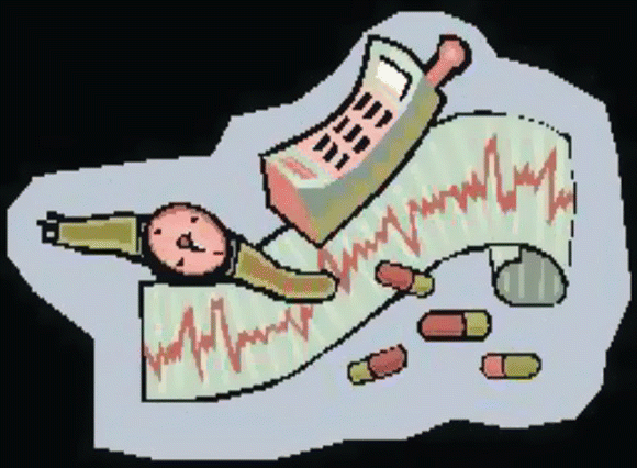
The treatment assignment was done by randomly dividing the group of subjects into three groups of eight people: one to receive Drug A, one to receive Drug B, and the third group to receive a placebo (labeled Drug C, for control).
If I had been involved in planning this experiment, I would have recommended that each subject’s heart rate be measured perhaps four times at 5 min intervals before the drug is administered and then afterward, as planned. This way, each subject would be its own control so that drug effects could be measured within subjects and evaluated against within-subject experimental error (à la the boys’ shoes experiment). This experiment, though, was done with a control group of subjects, so in the experiment under consideration, the drug effects will have to be evaluated against among-subject variability.
The data for this experiment are given in Table 7.10.
Table 7.10 Heart Rate Data. a
Source: Reproduced from Milliken and Johnson (2009, Table 26.4, p. 506), with permission of Chapman and Hall/CRC Press.
| ç | Drug | t1 | t2 | t3 | t4 |
| 1 | A | 72 | 86 | 81 | 77 |
| 2 | A | 78 | 83 | 88 | 81 |
| 3 | A | 71 | 82 | 81 | 75 |
| 4 | A | 72 | 83 | 83 | 69 |
| 5 | A | 66 | 79 | 77 | 66 |
| 6 | A | 74 | 83 | 84 | 77 |
| 7 | A | 62 | 73 | 78 | 70 |
| 8 | A | 69 | 75 | 76 | 70 |
| 9 | B | 85 | 86 | 83 | 80 |
| 10 | B | 82 | 86 | 80 | 84 |
| 11 | B | 71 | 78 | 70 | 75 |
| 12 | B | 83 | 88 | 79 | 81 |
| 13 | B | 86 | 85 | 76 | 76 |
| 14 | B | 85 | 82 | 83 | 80 |
| 15 | B | 79 | 83 | 80 | 81 |
| 16 | B | 83 | 84 | 78 | 81 |
| 17 | C | 69 | 73 | 72 | 74 |
| 18 | C | 66 | 62 | 67 | 73 |
| 19 | C | 84 | 90 | 88 | 87 |
| 20 | C | 80 | 81 | 77 | 72 |
| 21 | C | 72 | 72 | 69 | 70 |
| 22 | C | 65 | 62 | 65 | 61 |
| 23 | C | 75 | 69 | 69 | 68 |
| 24 | C | 71 | 70 | 65 | 63 |
a Table entries are the heart rates at 5 min intervals for each subject after taking the indicated drug.
Analysis 1: Plot the data
The data are shown in Figure 7.7, which is a connected scatter plot of pulse rate versus time, by drug and subject. (The data points are linked by subject. Subject is included in the plots only because if there were any outliers in the data, this would help identify the particular subject.)
Figure 7.7 indicates that Drug A subjects had a rising and falling pulse over the 20 min test period, while Drug B is elevated (compared to the control group, C) over the whole period. The mostly consistent rise and fall of pulse rate for all eight subjects over the four tests, though, seems a little unusual. The placebo, Drug C, as would be expected of a proper placebo, shows a generally flat pattern and at a lower average pulse rate than Drug B. These differences can be better seen in the interaction plot for drugs and time (averaged over subjects) in Figure 7.8

Figure 7.8 Average Pulse Rate versus Time by Drug.
Figure 7.8 shows considerable interaction: the average pulse rate versus time patterns are markedly different for the three drugs.
The ANOVA structure for this experiment is the same as for the corrosion-resistance split-unit experiment (under certain simplifying assumptions about the variation across time periods within subjects). At the subject level, the design of this experiment is a completely randomized design with three treatments, each applied to eight experimental units. Within each drug, there is a two-way classification of the responses, subjects (8) by times (4). The ANOVA will have two error terms: among subjects (Error1) and within subjects (Error2). Table 7.11 gives the ANOVA and confirms what our eye sees. The significant drug by time interaction confirms the Figure 7.8 visual impression that the drug effects over time are not at all consistent over the three drugs; they are not just manifestations of the random variability among subjects.
Table 7.11 ANOVA for Drug/Pulse Rate Experiment.
| Source | df | SS | MS | F | P |
| Drug | 2 | 1333 | 666.5 | 6.0 | .009 |
| Error1 | 21 | 2337 | 111.3 | 15.0 | .000 |
| Time | 3 | 290 | 96.5 | 13.0 | .000 |
| Drug × time | 6 | 527 | 87.9 | 11.8 | .000 |
| Error2 | 63 | 469 | 7.5 | ||
| Total | 95 | 4957 |
If the purpose of the drugs was to elevate pulse rate, the interaction plot shows that both drugs were successful but Drug B achieves that increase earlier and longer than does Drug A.
Discussion
Some of the experimental situations in the previous chapters could have been addressed with a repeated measures design. For example, consider the market research objective in Chapter 4. The objective was to compare the effects of three store displays on shampoo sales. A completely randomized design was used in which 15 stores were selected for the experiment, and each display was randomly assigned to five stores. An alternative way to design the experiment would be to have each of the 15 stores run the three displays successively with a protocol that specifies an appropriate time lag between displays. Because order could have an effect, the six different orders could be assigned in a balanced way: three of the orders could be assigned to two stores each, and three of the orders could be assigned to three stores each. Or, the experiment might have been done with either 12 or 18 total stores to keep things balanced.
In the present chapter, the Latin square experiment involving cars, drivers, and additives can be thought of as a repeated measures design. Each driver was subjected to a sequence of car/additive combinations. Learning or boredom effects were a concern in this experiment.
Extensions
An extension of the drug/heart rate experiment would be to repeat the experiment with the same subjects but assign each group to another drug. This could be done again so that every subject is tested against all three drugs. The time between each test (and its four pulse rate measurements) would be long enough to dissipate the effects of the previous drug. This is a crossover design (Cochran and Cox 1957; Ohlert 2000). This class of designs is often used in agricultural experiments. For example, plots of land in a tomato field that got Fertilizer A this year would get Fertilizer C next year, and vice versa.
Robust Designs
Introduction
The concept of robustness and the role of designed experiments were mentioned in the coating material experiment earlier in this chapter: the goal was to implement a curing process that is insensitive to curing-temperature variations within a range that a coating purchaser is able to control to in its use of the material. The coating would have good corrosion resistance as long as the curing temperature is kept within the specified limits. Demonstrating or achieving robustness is also an objective in several examples in the preceding chapters. Producers of crop seed or fertilizers want to be able to demonstrate that their product is effective in a variety of growing conditions, so a randomized block experiment, where blocks span anticipated growing conditions, provides a means of evaluating product robustness with respect to growing conditions. Producers of a fuel additive would like the benefit of that additive (reduced emissions) to be robust to driving conditions, so tests, defined by a Latin square design, were conducted using multiple cars and drivers to evaluate different additives and their robustness of emission control to variation of cars and drivers. As I have tried to stress, experiments don’t end with an ANOVA and its P-values. It is what is learned and how that learning can be used to improve products, processes, and programs that is the real payoff. Experiments that are aimed at achieving robustness are an important category of experiments. This section deals with a particular approach to designing experiments aimed at demonstrating robustness or finding sources of nonrobustness.
Variance transmission
Robustness can be expressed in terms of designing a system or process in order to minimize the variability of its output. Figure 7.9 illustrates this graphically for the design of a pendulum to be used, say, in a grandfather’s clock. There is a mathematical, physics-based relationship between the period of a pendulum (the time for one swing) and the pendulum’s length. The curved line in Figure 7.9 depicts that relationship; note that the curve is plotted on a semi-log scale. Pendulums can vary in length, just due to manufacturing variability, as represented by the probability distributions along the horizontal axis. The variability of lengths is transmitted, mathematically into variability of the pendulum’s period, as shown along the vertical axis. Gears in the clock translate the pendulum’s motion to movement of the clock hands that tell us what time it is (I assume that readers have seen clocks with hands). A manufacturer will have spec limits on clock accuracy, so high variability of the pendulum’s period among clocks, due to variation in the pendulum lengths, would mean that more clocks would fail the specs and have to have their pendulums replaced.

Figure 7.9 The Transmission of Variation in the Length of a Pendulum to Variability of the Pendulum’s Period. .
Source: Reproduced from BHH (2005, p. 551), with the permission of John Wiley & Sons
To minimize variability of the pendulum’s period, the message from Figure 7.9 is that the pendulum should be as long as possible. Size matters. (Can I say that?) Note that the transmitted variation at x = 10 cm is considerably less than it is at x = 2 cm. That’s (in part) why tall grandfather clocks cost more than short ones or table clocks.
In this example, the mathematical relationship between system performance (y) and one particular design variable (x) is known from physics. In more general and more complex situations, the relationship between system performance and system design is not known. As an example, in the case study in Chapter 1, the relationship between the locations at which a wire bond was pulled to measure pull strength was not known. Designed experiments, though, were conducted, in essence, to estimate that relationship and then use the findings to better control the testing process.
In the 1980s, the concept of robust design received a lot of attention, thanks to the work of Genichi Taguchi (1991). He recommended a variety of designed experiments and data analyses that would lead to the design and manufacture of robust systems. Taguchi’s methods would find the design parameters that would minimize the variability of system output in a variety of situations. Conferences were held by statisticians to understand and critique these statistical methods.
One example I remember hearing at the time is the following: a manufacturer of ceramic pots was experiencing a high rate of breakage (sound familiar?). Investigation led to the finding that the oven in which the pots were baked had a very uneven temperature distribution (sound familiar?). The solution proposed was to buy a new and better oven that would provide a more uniform temperature throughout. This would be a very expensive solution. However, process engineers, through experimentation with the ceramic design parameters (perhaps guided by Professor Taguchi, I don’t remember), found that by increasing the amount of ash in the clay, the pots became less temperature sensitive (more robust to temperature differences), so less breakage occurred. Ash is cheap, so this was a much less expensive solution. A celebration ensued and bonuses were paid (I’m making that part up).
Taguchi experimental designs aimed at determining robust processes or products have the following structure. First, known or potential factors (or variables) that affect a product’s performance need to be identified. These factors fall in two categories:
- Control factors. These are characteristics of the product, such as dimensions and materials, that the designer has control of and that will ultimately define the product.
- Noise factors. These are possible influences on product performance outside of the designer’s control, such as environmental conditions or uncontrolled and unavoidable deviations in product characteristics such as the variation of pendulum lengths in Figure 7.9.
Then, a Taguchi experimental design is as follows: first, choose an “inner array” of design factors. These arrays are generally factorial or fractional factorial combinations of two- or three-level design factors.
Next, an “outer array” of noise factors is determined—again, usually two- or three-level factorial or fractional factorial combinations of the noise factors.
Then, the complete set of experimental conditions is obtained by running the outer array of noise factors at each combination of design factors in the inner array.
Figure 7.10 illustrates this compounding of inner and outer arrays graphically.

Figure 7.10 An Inner 3 × 3 Array of Two Design Factors and an Outer 23 Array of Three Noise Factors. .
Source: Reproduced from BHH (2005, p. 553), with the permission of John Wiley & Sons
In Figure 7.10, there are a total of 9 × 8 (=72) treatment combinations in the experiment. Depending on how the experiment might be conducted, there might be blocking, replication, or unit splitting in the conduct of the experiment. Statistical analysis would need to reflect these aspects of the experiment.
Now, how should the data be analyzed to determine the most robust set of design factors? This is where Taguchi methodology departs from convention by calculating “signal-to-noise” summary statistics at each design combination and then picking the combination of control factors that maximizes signal to noise. Further experimentation might be done to refine the choice.
For the experimental array in Figure 7.10, the signal-to-noise analysis might be as follows:
- Calculate ybar and s, the mean and standard deviation of the eight responses at each of the nine combinations of design factors.
- Calculate the relative standard deviation, s/ybar, at each of the nine settings of design factors. This is a particular noise-to-signal ratio.
- Choose the combination with the smallest relative standard deviation. Possibly conduct further experimentation and analysis to refine and confirm the choice of design factor levels.
To illustrate an alternative to the Taguchi signal-to-noise approach, I need to commit a little bit of mathematics.
Mathematical model: Robustness
Process output, y, is a function of design factors and noise factors, expressed as follows:
where x is a set of control factors and w is a set of noise factors; w can be controlled in an experiment, not in use.
The nature of f(x,w) determines how variability of w will be transmitted into variability of y, which means variability of product performance, which means quality and customer satisfaction, good or bad. Thus, the experimental design and subsequent data analysis will be aimed at estimating this relationship. That estimate will then provide a means of finding the x settings that are most robust to variation in w. Here is a simple illustrative example.
Consider a situation in which there are two control factors, x 1 and x 2, and one noise factor, w. Suppose the statistical relationship between a response variable, y, and these three factors is:

where e is the effect of additional noise factors, not controlled in the experiment. In use, both e and w are random variables.
Note that the cross-product term in this model, dx 2 w, means that the effect of x 2 on y is amplified by w. There is interaction between these two factors, in the statistical sense: the effect of x 2 on y is different for different values of w.
By using the properties of sums of random variables and the product of a constant and a random variable, under the aforementioned model, the variance of y is
Thus, to minimize the variance of y, x 2 needs to be chosen to minimize (c + dx 2)2. If feasible, the optimum choice, as a little algebra shows, is x 2 = −c/d, in which case w has no effect on the variation of the process output. If this solution for x 2 is not feasible, the optimal choice of x 2 would be the feasible value of x 2 that minimizes |c + dx 2|. The experiment and data analysis would provide estimates of c and d from which the most robust x 2 setting would be determined.
What about x 1? Its effect on y is not affected by w, so x 1 can be dialed up or down so that the performance characteristic will meet its target value and not transmit additional variation. In our pendulum example, once the pendulum length has been specified, gear ratios can be adjusted appropriately so that the clock keeps accurate time.
Robust design is sometimes said to “capitalize on interaction.” This simple example illustrates how that can be done.
Concluding comments
There are many contexts in which robustness is an important design goal. Questionnaires needed to be worded clearly, so that confusion and misinterpretation do not cloud the results. Products need to operate reliably in a range of operating conditions. Online systems for signing up for health insurance need to be capable of coping with variations in demand and user needs and capabilities, etc. Designed experiments and appropriate data analysis and communication of results help achieve robust products and processes. Taguchi and subsequent researchers and practitioners in the United States (see, e.g., Phadke 1989; Wu and Hamada 2000; Wikipedia (2014a)) encouraged a heightened focus on product and process robustness that needs to be widely recognized.
Optimal Designs
Introduction
For the most part, the experiments used to illustrate the design families in this book have come to us fully formed with respect to choices of treatment and blocking factors, the number and levels of these factors, the combinations of factors that are included in the experiment, the number of replications, and the responses and ancillary variables that were measured. I have indicated that subject-matter knowledge and issues, along with statistical and economic considerations and even personalities, must interact to make these key design decisions in order to have some assurance before the experiment that the experiment has the capability of answering pertinent questions. For example, in the ethanol experiment in Chapter 5, we took it on faith that the experimenters had identified two important and pertinent x-variables that might influence CO emissions from automobiles. We did have some knowledge from the literature that the ranges of the x-variables were reasonable. We do not know, however, why the experimenters chose to run two replications of a 3 × 3 set of treatment (x-variable) combinations. It could have been cost; it could have been that previous, related work had found that a second-order polynomial at least roughly described the relationship between the x-variables and CO emissions. It could be that they saw this design in another textbook.
There are of course many other suites of treatment designs that could have been run. For example, a response surface design with a 2 × 2 factorial set of points, plus four radial points, plus a center point would again make for a total of nine treatment combinations. The levels that define the 2 × 2 points and the star points would be other design options. The nine selected treatment combinations could all have been replicated twice for 18 runs. Or, a 4 × 4 set of points, with only one replication, plus two center points, would have been another way to distribute 18 treatment design points around the selected x1 − x2 region. And, of course, there is probably no strong reason to make exactly 18 runs, so the possibilities are endless.
For the most part, in this book, we have considered experimental designs with rectangular experimental regions—multifactorial structures. Nature and theory are not always this neat and tidy. There will be constraints that preclude the designs, both treatment designs and experimental designs, that we have discussed and illustrated. Active research in this area is aimed at finding optimal designs that incorporate specific constraints and objectives in determining an experimental design. This approach is better than trying to force a basic design into a constrained situation. Once again, statisticians have risen to the occasion of finding designs that better fit real-world situations.
Finding “optimal experimental designs”
Statistical and computational tools exist for evaluating candidate designs. These start with various measures of the precision of estimates and predictions that would be obtained from the experiment. Estimates and predictions generally depend on the nature of the function ultimately fitted to the experiment’s data—the model. But we don’t necessarily know that function, you say. That’s why we’re running the experiment, for goodness’ sakes! Relax. For planning purposes, we always make some assumptions. This is directly analogous to the sample size analyses we did in earlier chapters in which we made assumptions, for example, about the error variance and the Normal distribution in order to determine how many observations we needed to achieve a desired confidence interval width or to meet power curve targets.
In the rat food example in Chapter 4, the scientists expected the relationship between growth rate and supplement amount to be linear. Under that assumption, the optimum design would be half of the runs at each end of the selected range of the x-variable. Prudence, though (she was the FLS involved in the study), led to a design with several intermediate x-values. We can, and should, in general, vary the assumptions and see how the design changes in response. Also, it should be pointed out that basic designs, such as a randomized block design with multifactor treatments, are also linked to particular statistical models.
Suppose, for planning purposes, that we assume that a second-order polynomial is a good approximation to the relationship in nature, or the laboratory experiment, between CO and x1 and x2. (“All models are wrong; some are useful,” said George Box.) Under this assumption, we know the mathematical function of the data by which the coefficients will be estimated and predictions will be calculated. We know the formulas for the precision of those estimates and predictions, up to the value of sigma. These formulas are all a function of the experimental design—the location of the design points and the number and locations of replications. We and our computers can do those calculations for every candidate design and compare the results and try to balance cost and precision. We (or your friendly, local statistician) could repeat the whole exercise for another candidate family, such as a bivariate log-linear model. Subject-matter knowledge and theory can identify candidate models. We might conjecture, also, that for planning purposes, if we choose a design that does a good job of fitting the second-order model, it might still be OK (robust enough) for fitting another model that we ultimately determine when we analyze the data. Methods for finding model-robust designs (as opposed to model-dependent designs) are an area of active research (see, e.g., Smucker, del Castillo, and Rosenburger 2011 and references).
This comparison of designs would be an unwieldy analysis, so statisticians have developed summary measures of a design’s “goodness.” These include:
- The average of the variances of the estimated coefficients
- The maximum of the variances of the estimated coefficients
- The maximum variance of predictions in a specified region of explanatory variables
These variances are all multiples of the experimental error variance; the multiplier is a function of the array of design points in the design.
Instead of evaluating a possibly large number of candidate designs, we can (let the computer) work the problem in reverse. We can give the computer a large number of possible design points, such as a fine grid of points in the x1 − x2 region of the ethanol experiment and then tell the computer, “I want to fit a quadratic model using only 18 points in this region. Find me the 18 points that minimize the maximum variance of predictions in the x1 − x2 region (criterion 3).” And, the computer will do it (see, e.g., JMP, jmp.com). We can repeat the process for n = 24 and 36, say, to see how the design changes and precision improves with these larger experiments and then consider cost–benefit trade-offs.
Experimental designs obtained in this way are sometimes called “computer-aided designs.” For a concise discussion of these designs, see the online NIST Engineering Statistics Handbook, Section 5.5.2 (NIST 2014). In addition to quantitative criteria for deciding on a model, graphical methods are also useful (Anderson-Cook, Montgomery, and Myers 2009).
Design augmentation
In several examples in this book, I discussed possible further experimentation that might be done to follow up on the results of the experiment under discussion. For example, a follow-up multifactor experiment might be conducted in an adjacent factor region. The present experiment would give an idea of the nature of the relationship between the response and the treatment factors, so one could use that information to specify a candidate set of additional treatment combinations and find the optimal design for augmenting the current data to best enhance the fit of the model fitted to the initial experiment.
Some other situations in which optimal, computer-aided experimental designs are valuable are:
- Constraints on the experimental region eliminate some points in a full or fractional array of block or treatment combinations.
- Block structures and sizes for conventional experiments may not be appropriate.
Computational resources, of course not available when the CRD and RCB design families and other designs in the preceding chapters were developed, provide a great opportunity for expanding the actual use of experimental design, which happens also to be the purpose of this book. For a case study-based introduction to optimal design and illustrations of the wide range of situations in which optimal designs can provide context-specific experimental designs, see Goos and Jones (2011). This book is written as a dialogue between the two authors, asking and answering questions that a reader might have. Another pertinent reference is Atkinson, Donev, and Tobias (2007). Wikipedia (2014b) provides an overview and additional references.
Assignment
Choose a topic of interest to you and an issue to investigate with an experiment. Develop three experimental designs for investigating this issue: (i) Latin square, (ii) split unit, and (iii) repeated measures. Discuss and compare your three alternatives. Show how you would plot the data and lay out the ANOVA tables for each.
References
- Anderson-Cook, C., Montgomery, D., and Myers, R. (2009) Response Surface Methodology: Process and Product Optimization Using Designed Experiments, 3rd ed., John Wiley & Sons, New York.
- Atkinson, A. C., Donev, A. N., and Tobias, R. D. (2007) Optimum Experimental Designs, with SAS, Oxford University Press, Oxford.
- Box, G., Hunter, W. G., and Hunter, J. S. (1978, 2005) Statistics for Experimenters, John Wiley & Sons, Inc., New York.
- Cochran, W., and Cox, G. (1957) Experimental Design, John Wiley & Sons, Inc., New York.
- Fisher, R. A. (1938) Presidential Address to the First Indian Statistical Congress, http://www.economics.soton.ac.uk/staff/aldrich/fisherguide/quotations.htm.
- Goos, P., and Jones, B. (2011) Optimal Design of Experiments: A Case Study Approach, John Wiley & Sons, Ltd, Chichester.
- Jones, B., and Nachtsheim, C. (2009) Split-Plot Designs: What, Why, and How, Journal of Quality Technology, 41(4): 340–361.
- Milliken, G., and Johnson, D. (2009) Analysis of Messy Data Volume I: Designed Experiments, 2nd ed., Chapman and Hall/CRC Press, Danvers, MA.
- NIST-SEMATECH (2014) Engineering Statistics Online Handbook, Section 5.5.2. http://itl.nist.gov/div898/handbook/.
- Ohlert, G. (2000) A First Course in Design and Analysis of Experiments, W. H. Freeman, New York.
- Phadke, M. (1989) Quality Engineering Using Robust Design, Prentice-Hall, Englewood Cliffs, NJ.
- Smucker, B., del Castillo, E., and Rosenburger, J. (2011) Exchange Algorithms for Constructing Model-Robust Designs, Journal of Quality Technology, 43, 1–15.
- Taguchi, G. (1991) System of Experimental Design: Engineering Methods to Optimize Quality and Minimize Cost, Quality Resources, White Plains, NY.
- Wikipedia (2014a) Robust Parameter Design, http://en.wikipedia.org/wiki/Robust_parameter_design.
- Wikipedia (2014b) Optimal Design, http://en.wikipedia.org/wiki/Optimal_design.
- Wu, C. F., and Hamada, M. (2000) Experiments: Planning, Analysis, and Parameter Design Optimization. John Wiley & Sons, Inc., New York.