6
Randomized Complete Block Design
Introduction
As discussed in Chapter 2, blocking of the experimental units in an experiment can be crucial to an experiment’s success and value. The choice of blocks defines the scope of the experiment and the conclusions it supports. Blocking can also increase the precision with which treatments are compared, relative to an unblocked experiment spanning the same set of experimental units. We will see later in this chapter a dramatic demonstration of the efficiency of the blocked design in the context of the boys’ shoes experiment in Chapter 3.
The randomized block design (RBD) is constructed like a collection of b separate completely randomized designs (CRD) for comparing k treatments, where b is the number of blocks. In each block, each of k treatments is randomly assigned to one or more experimental units, as in a CRD. In the simplest situation, the number of treatments equals the number of experimental units (eus) in a block, so each treatment is assigned to only one eu in each block. (As discussed later (p. 203), it is possible for there to be fewer than k eus in a block, so that not all treatments can be run in each block.) We have already seen an example of this type of a randomized block experiment: the aforementioned boys’ shoes material experiment in Chapter 3. In that experiment, there were 10 blocks (boys), each of which (whom) contained two experimental units (feet). The two treatments, shoe sole materials A and B, were assigned randomly to the two feet in each block. Of course, no single block could be analyzed as a CRD because there was no replication—there was only one replicate of each treatment in a block. However, the collection of wear differences, (B–A), across boys, was a set of replicate differences and thus could be statistically analyzed, as in Chapter 3.
In other situations, one can have blocks that have enough eus so that each treatment can be randomly assigned to two or more eus in each block. For example, in an experiment to evaluate the effects of medication on cholesterol levels, the blocks may be groups of people categorized by sex and three age groupings. One might have 60 participants in each of these six blocks and randomly assign 20 (eus) in each block to one of three medications, say lipitor, zocor, and the ever-popular placebo. Cholesterol measurements would be made at the beginning of the trial and periodically during the trial. Other participant characteristics such as weight and body mass index would also be measured initially and periodically. The response that might be measured and analyzed could be the change in cholesterol levels between final and initial measurements. Other analyses could evaluate how quickly a medication led to a change in cholesterol.
In this sort of experiment, we can evaluate treatment differences in each block, and moreover, we can evaluate whether the treatment differences are consistent across participant groups, that is, from block to block. In more technical terms, we can test for “block–treatment interaction.”
The RBD can have unequal replication (of treatment assignments within blocks), but for convenience, we will restrict our attention here to equal replication, say, r replicates of each treatment in each block. We start with the general case of two or more replicates of each treatment in each block and then address the special case of single replicates for each treatment in a block.
Design Issues
The first issue to deal with is whether the experiment should be blocked or not. Blocks serve several purposes in a design, as discussed earlier. Are there natural blocks of experimental units that we are interested in? For example, men and women subjects in a clinical trial. Do we want to use blocks to determine the range of applicability of the experiment’s results (e.g., different growing conditions in an agricultural experiment, different sources of raw materials used in an industrial process, different regions in a marketing experiment)? Is there a source of variation that we can control by blocking (e.g., time of day in a production process)? Are there experimental objectives that call for the inclusion of particular blocks (e.g., multiple suppliers of an automobile part)?
Once the decision has been made to structure or group the experimental units into blocks, the next design issues pertain to the number and nature of the blocks and the number of experimental units in each. If we have freedom to control the number of eus in a block, a control we didn’t have with the boys’ feet, but did with the cholesterol medication experiment in the previous section, then the choice of block size will depend on the number of treatments to consider in the experiment and the number of replicates in each block. Power and sample size calculations can be used to help size the experiment.
RBD with replication: Example 1—battery experiment
Montgomery (2001, Chapter 5) provides data from an experiment that addresses the effect of temperature on battery life. The following story wrapped around the data is mine.
The government, for a special (perhaps secret) application, needs to power an electronic device with a battery that will provide power for a specified duration and do so reliably over a wide range of temperatures. Three contract bidders have each produced 12 prototype batteries for testing by the government agency (these are expensive, government-procured batteries, not household batteries, and that is the reason for the small size of this experiment). These batteries differ primarily in their plate material: denoted here, for the sake of security, as materials 1, 2, and 3. Thus, there are a total of 36 experimental units, structured as three blocks of 12 eus each.

The treatments to which these batteries will be subjected are defined by operating temperature. The government’s requirement is that the batteries have “reliable operation” over temperatures ranging from 15°F (degrees Fahrenheit) to 125°F. The agency has decided to test at those extremes and the midrange; thus, the selected temperature levels are 15, 70, and 125°F. (Note: My former employer, Sandia National Laboratories, operates a Battery Abuse Testing Laboratory, known coolly as the BATLab, and they could do this testing and more. Note the many other possibilities: a camera abuse testing laboratory would be a CATLab, etc.)
Four batteries in each block are randomly assigned to each temperature. The batteries are connected to a specified load while operating at their assigned temperature. We’re not told, but will assume that storage conditions are applied independently to each battery in the experiment. We will also assume that the temperatures are tightly and accurately controlled. During the test, the batteries are continually monitored and their lifetime, in hours (or possibly a coded response, you can’t be sure), is the recorded response. Lifetime is operationally defined as the time at which battery output falls below a specified level.
As noted in Chapter 2, some authors, for example, the author of the Wikipedia (2014a) entry on RBD, describe blocking factors as “nuisances”—extraneous sources of variation that the design controls in order to improve the precision with which treatments can be compared. That is decidedly not the case of the blocks in this experiment. The blocks are the three manufacturers, and the government is most interested in choosing among these three battery makers. This experiment’s design is an RBD because of the way in which the eus (batteries) are grouped and the treatments (temperatures) are assigned to eus. Whether the blocking factor (or factors) are nuisances or of keen interest doesn’t change the experimental design; it would, however, affect the focus of the analysis.
The results of this experiment are shown in Table 6.1.
Table 6.1 Battery Lifetimes by Material and Temperature.
| Material | Temperature (°F) | ||
| 15 | 70 | 125 | |
| 1 | 130 | 34 | 20 |
| 74 | 80 | 82 | |
| 155 | 40 | 70 | |
| 180 | 75 | 58 | |
| 2 | 150 | 136 | 25 |
| 159 | 106 | 58 | |
| 188 | 122 | 70 | |
| 126 | 115 | 45 | |
| 3 | 138 | 174 | 96 |
| 168 | 150 | 82 | |
| 110 | 120 | 104 | |
| 160 | 139 | 60 | |
Table 5.1, p. 176 of Montgomery (2001), reproduced by permission of John Wiley & Sons.
Analysis 1: Plot the data
Because the treatment factor (temperature) is a quantitative variable and the blocking variable is a qualitative variable (plate material), the appropriate display of the data is a plot of lifetime versus temperature for each material. This plot is shown in Figure 6.1.

Figure 6.1 Scatter Plot of Battery Lifetimes versus Temperature, by Material.
Figure 6.1 shows that temperature, especially high temperature (125°F), substantially shortens battery life, relative to low-temperature (15°F) storage. The lifetimes versus temperature trends, though, differ considerably by material. Material 1 is degraded substantially at 70°F, while material 3 is not affected at all at 70°F (relative to life at 15°F). Material 2 is intermediate—some degradation from 15 to 70°F and additional degradation at 125°F.
It is clear that if we have to pick a material based on this experiment, material 3 is the winner: batteries with this material have the longest lifetimes at both 70 and 125°F and lifetimes at 15°F that are comparable to those for the other two materials.
Figure 6.1 shows (eyeball analysis—never underestimate the value of eyeball analysis) that the variability among batteries, of each material, that are exposed to the same temperature is pretty consistent across temperatures and materials. Thus, we collapse the data in each material/temperature combination and display the averages in an interaction plot: Figure 6.2. Note, though, that in contrast to the previous chapter which dealt with interaction among treatment factors, here, we are dealing with block by treatment interaction. Just to reiterate: material, or manufacturer, is a blocking factor; it defines groups of experimental units. It is not a treatment applied to an experimental unit.

Figure 6.2 Interaction Plot of Material/Temperature Means.
As discussed in Chapter 5, (statistical) interaction between two factors, in this case plate material and temperature, occurs when the effect of one factor is different for the different levels of the other factor. That is distinctly the case here, at least graphically, because 70°F apparently affects material 1 batteries quite differently (average lifetime is cut in half) than it does for the other two materials.
Analysis of variance
To address the question of whether the apparent interaction is “real or random,” ANOVA is again the tool. For the randomized complete block design with replication, the ANOVA has the structure shown in Table 6.2.
Table 6.2 ANOVA Structure for Randomized Complete Block Design with Replication.
| Source | df | SS | MS | F | P |
| Blocks (B) | b − 1 | ||||
| Treatments (T) | t − 1 | ||||
| B × T interaction | (b − 1)(t − 1) | ||||
| Error | bt(r − 1) | ||||
| Total | btr − 1 |
This is the very same ANOVA structure, a “two-way ANOVA” with replication, as in the case of a CRD with a crossed two-factor treatment structure and r eus for each treatment combination (e.g., the poison/antidote experiment of Chapter 5). Though the ANOVAs are the same mathematically and data tables would look the same, this should not confuse you into thinking the experiments are the same. In Chapter 5, we had one group of homogeneous eus and did one randomization of the assignment of the (two-factor) treatment combinations to eus. The design was a CRD. Here in Chapter 6, we have b different types/blocks of experimental units, and we do separate randomization of treatments to eus in each block—this is an RBD.
Note that the Error term in Table 6.2 is the variability of the r eus in each block–treatment combination, pooled across the bt block–treatment combinations. There are bt block–treatment combinations and r − 1 df for experimental error in each set of r replicates; hence, the Error df is bt(r − 1).
The ANOVA for the battery lifetime data is shown in Table 6.3.
Table 6.3 ANOVA for Battery Experiment.
| Source | DF | SS | MS | F | P |
| Material | 2 | 10 684 | 5342 | 7.91 | .002 |
| Temp | 2 | 39 119 | 19 559 | 29.0 | .000 |
| Interaction | 4 | 9614 | 2403 | 3.56 | .019 |
| Error | 27 | 18 235 | 675 | ||
| Total | 35 | 77 647 |
The pertinent result to consider first in Table 6.3 is the test for interaction because if interaction is significant, the message of that finding is that you should not compare materials averaged across temperatures; the temperature effects are not the same across materials. The interaction test result for these data is F = 3.44 on 4 and 27 df, and a P-value of .02. This is fairly strong evidence that the apparent interaction is real: the temperature effects are not the same for all three materials. The ANOVA confirms the eyeball impression.
But so what? Can we choose a winning battery from this result? Well, it depends. (Statistical) Life doesn’t end with a significance test. We don’t know the requirements a battery is supposed to meet. If the requirement was that the battery should last 1 h, reliably, over the entire temperature range, then all three battery types meet this requirement, comfortably (with perhaps a little concern about materials 1 and 2 at 125°F—see Fig. 6.1). We could choose the contractor based on cost or Congressional district—whatever.
On the other hand, if the requirement was that the battery should last 50 h reliably (meaning with high probability), over the entire temperature range, then none of the battery types looks adequate.
Reliability analysis
The best battery at 125°F is material 3, which had an average lifetime (over the four batteries tested) of 85.5 h. The variability among batteries of the same type at a given temperature is estimated by the square root of the Error MS in Table 6.1: ![]() . For the sake of estimating battery reliability (for this example, reliability is defined as the probability that battery life exceeds 50 h), let’s use the statistical model that lifetime has a Normal distribution with a mean of 85.5 h and a standard deviation of 26 h. Then, the estimated reliability is Prob(z > (50 − 85.5)/26) = Prob(z > −1.36) = .91, where z has a standard Normal distribution (mean = 0, stdev = 1.0). Thus, as a point estimate, about 9% of material 3 batteries would fail to provide 50 h of life at 125°F. This may not be good enough for the government. Furthermore, because the mean lifetime is only based on four observations, this is a pretty imprecise estimate. We need further analysis to account for this imprecision, such as follows.
. For the sake of estimating battery reliability (for this example, reliability is defined as the probability that battery life exceeds 50 h), let’s use the statistical model that lifetime has a Normal distribution with a mean of 85.5 h and a standard deviation of 26 h. Then, the estimated reliability is Prob(z > (50 − 85.5)/26) = Prob(z > −1.36) = .91, where z has a standard Normal distribution (mean = 0, stdev = 1.0). Thus, as a point estimate, about 9% of material 3 batteries would fail to provide 50 h of life at 125°F. This may not be good enough for the government. Furthermore, because the mean lifetime is only based on four observations, this is a pretty imprecise estimate. We need further analysis to account for this imprecision, such as follows.
The standard error of the estimated mean is ![]() , based on 27 df. The t-value for the .025 point on the t(27) distribution is −2.05. Thus, the lower 97.5% confidence limit on mean lifetime for material 3 at 125°F is given by 85.5 − 2.05(13) = 58.9. By using this conservative value of 58.9 h for the mean and 26 h as the standard deviation, the estimated probability of exceeding 50 h life is Prob(z > (50 − 58.9)/26) = Prob(z > −.34) = .63. Thus, conservatively (with ~97.5% confidence in this illustration), as many as 37% of material 3 batteries could fail to meet the requirement. (This calculation is a little bit optimistic because we have not accounted for the imprecision in the estimated standard deviation, but, even with a bit of optimism, the basic conclusion is that we definitely have a reliability problem.)
, based on 27 df. The t-value for the .025 point on the t(27) distribution is −2.05. Thus, the lower 97.5% confidence limit on mean lifetime for material 3 at 125°F is given by 85.5 − 2.05(13) = 58.9. By using this conservative value of 58.9 h for the mean and 26 h as the standard deviation, the estimated probability of exceeding 50 h life is Prob(z > (50 − 58.9)/26) = Prob(z > −.34) = .63. Thus, conservatively (with ~97.5% confidence in this illustration), as many as 37% of material 3 batteries could fail to meet the requirement. (This calculation is a little bit optimistic because we have not accounted for the imprecision in the estimated standard deviation, but, even with a bit of optimism, the basic conclusion is that we definitely have a reliability problem.)
This (low reliability) is bad news. It’s back to the drawing board for the battery manufacturers. Or, hmm. Maybe it’s worth reexamining the requirements. This happens in practice. Do we really need 50 h of reliable life? And just how high a reliability do we really need? And how likely is it that the device will really be required to operate at 125°F? Government (and other) agencies have been known to set “stretch requirements” for systems and devices in order to build in some margin (after all, field operation will be different from battery testing in a controlled environment). Contract bidders have been known to ask that the requirements be “scrubbed” a bit. “Let’s sharpen our pencils,” they say. The discussion could get contentious, but at least all parties have data to work from. And the discussions could lead to additional testing; the data obtained in this experiment could be used to help decide how much testing should be done. As we discussed in the case of the boys’ shoes (Chapter 3), integrity is needed as well as statistical and battery design and manufacturing skills to assure that the government gets the battery it needs at a price that doesn’t gouge the taxpayer.
Further analysis
Let’s suppose the government decides to drop the battery made with material 1, with its poor performance at 70°, from consideration. How do materials 2 and 3 compare? Graphically, they have a similar pattern, but material 3 batteries have longer lifetimes at the two higher temperatures. Is the difference real, or could it be random?
Table 6.4 gives the ANOVA for the battery life data, excluding material 1.
Table 6.4 ANOVA for Battery Experiment: Materials 2 and 3.
| Source | DF | SS | MS | F | P |
| Material | 1 | 1683 | 1683 | 3.68 | .07 |
| Temp | 2 | 30 231 | 15 115 | 33.1 | .00 |
| Interaction | 2 | 2537 | 1268 | 2.78 | .09 |
| Error | 18 | 8226 | 457 | ||
| Total | 23 | 42 677 |
Table 6.4 shows some evidence of interaction and some evidence of a real difference between materials, averaged over temperatures (which is appropriate if you assume interaction is negligible). A cautious government agency would call for further experimentation to better resolve the difference between materials 2 and 3.
Bringing subject-matter knowledge to bear
The alert reader will have noticed that temperature is a quantitative treatment factor and our analysis thus far has not made use of that characteristic. The analysis has helped the sponsoring agency decide to eliminate material 1 from further consideration and to conduct further experiments to sharpen the difference between materials 2 and 3, and that may be enough. Further analysis aimed, for example, at linking battery lifetime to temperature via a mathematical function is not really needed. For designing further experiments, though, considering such a relationship may be helpful. This experiment also provides an opportunity to bring in some subject-matter theory to the analysis, which is always a good idea.
Chemical reactions, such as occur in the discharge of a battery, are often accelerated by temperature. That is why the battery lifetimes in this experiment decrease with increasing temperature. The theory underlying this phenomenon has led to what is called an Arrhenius equation (Wikipedia 2011). Under this theoretical relationship, the logarithm of lifetime is a linear function of the reciprocal of “absolute temperature.” Absolute temperature is measured on what is called the Kelvin temperature scale. Its “zero point” is absolute zero, where no thermal activity occurs. By way of contrast, the Celsius (or Centigrade) temperature scale has its zero point at the freezing temperature of water. The relationship between these two temperature scales is that absolute temperature = 273 + Celsius temperature. For example, 20°C is equal to 293°K.
The temperatures in the battery experiment are expressed on the Fahrenheit scale (which has its zero point at 32° below the freezing point of water). Converting the Fahrenheit temperatures to Celsius and then adding 273 reexpresses the experiment’s temperatures on the Kelvin scale. The Arrhenius equation uses the reciprocal of absolute temperature. Table 6.5 shows the conversion from Fahrenheit temperatures to Kelvin temperatures and then the reciprocal of Kelvin temperatures. The latter is labeled TKinv.
Table 6.5 Fahrenheit Temperatures Converted to Centigrade, Kelvin, and the Reciprocal of Kelvin Temperature.
| Temp (°F) | Temp (°C) | Temp (K) | TKinv |
| 15 | −9.4 | 263.6 | .038 |
| 70 | 21.1 | 294.1 | .034 |
| 125 | 51.7 | 324.7 | .031 |
The Arrhenius relationship refers to the rate of a chemical reaction. The battery characteristic measured is lifetime, not reaction rate. Lifetime and reaction rate are related, at least conceptually, because if the reaction rate doubles, the lifetime, that is, the time for the battery to discharge all of its stored energy, would be reduced by a factor of two. Thus, if the Arrhenius equation applies to these batteries, a plot of the logarithm of lifetime versus inverse absolute temperature would be approximately linear. However, we don’t know how lifetime was measured in this experiment. It could have been the time at which output voltage dropped below a particular threshold, not when it went to zero. Output voltage is not a linear function of remaining charge (as I learned from Wikipedia), so this measure of lifetime might not follow the Arrhenius relationship. We need to look at the data and see what the relationship is.
Figure 6.3 shows a plot of the average log-lifetimes versus inverse absolute temperature, by material. (This plot is essentially the mirror image of the earlier interaction plot—Figure 6.2—because, as can be seen in Table 6.5, TKinv is nearly a linear function of the experimental temperatures, in degrees Fahrenheit. In Figure 6.3, temperatures decrease from left to right.)

Figure 6.3 Plot of Average Log-Lifetimes versus Inverse Absolute Temperature.
If the Arrhenius relationship applied, we would expect to see roughly three straight lines, perhaps differing in slope. The slopes would differ if the different plate materials had different “activation energies,” in Arrhenius terminology. (In more general terms, the materials would have different temperature sensitivities.) No such pattern is exhibited. When separate straight-line regression models are fitted to each material’s data separately, only material 3 is statistically consistent with a straight-line model.
In this case, some subject-matter knowledge did not help us interpret the data. Clearly, we don’t know enough about this experiment and its data to push this analysis further. Perhaps the follow-on experiments can be built to a greater extent on appropriate battery chemistry theory.
Example 2: More tomato fertilizer experiments
Garden experiments
The experimenter in Chapter 3 soon realizes that getting a definitive comparison of tomato fertilizers out of her garden alone is difficult. She doesn’t have room to plant many tomato plants, and there is enough plant-to-plant variability among tomato yields that it is difficult to detect important differences in yield among the fertilizers she has in her experiment. One way to get more replication is to repeat her experiment year after year, but who has time for that? She has an inspiration: I’ll get other gardeners to join me in the experiment. She goes to a tomato-grower online chat room and soon finds 10 other people scattered around the country who are interested. They work out a protocol and eventually decide that they will each plant 10 tomato plants of one variety (not necessarily the same for all 11 experimenters—a possible expansion of the experiment) and randomly assign five plants each to fertilizers A and C. Thus, taken together, the experimental design is an RBD with 11 blocks, two treatments, and five replications of each treatment in each block. Plotting and analyzing the combined data (crowdsourcing?) would tell the tomato-growing group (and readers of their online report) whether there was a consistent difference between fertilizers across locations and whether that difference was real. It might also show interaction, which could mean that the winning fertilizer and the margin of victory were location dependent, which could lead to more experimentation as science marches on.
Product research experiments
A research organization charged with developing new and better fertilizers (perhaps more environmentally friendly) will want to run experiments that compare a new fertilizer to fertilizers on the market. The new fertilizer will have a broader, more profitable market if it can be shown that the new fertilizer consistently produces better yields and less harmful environmental effects than the competition in a wide variety of soil types and growing conditions. Thus, a blocked experiment is called for: choose locations (blocks) that span a suitable range of soil quality and growing conditions and at each location randomly assign fertilizers to plants, follow a good and consistent experimental protocol, and analyze the resulting yields. Because small differences in yield can have large economic effects, conduct a large enough experiment so that these differences can be estimated with good precision.
Example 3: More gear teeth experiments
Problems found in automobiles often result in recalls: owners are notified of the problem and advised to bring in their cars for corrective service, paid for by the manufacturer (at the time this is written, General Motors has had a massive recall of ignition switches). The story (my story) in Chapter 4 was that broken teeth are caused by low injection volumes of gear material into the gear mold. We don’t know if that problem had existed from the start of production, or if it is more localized. The set of tests in Chapter 4 did not identify the gears by production date. Now, ideally, the auto company could visit their supplier, say, “Let’s work together on this,” and ask for their production records: “You do keep records on how much powder was used in each production run, don’t you?” Of course, even if you know when underweight gears were produced, you don’t necessarily know in what cars they were installed. Major parts have serial numbers that can be tracked, small plastic gears don’t. So, the auto manufacturer may not be able to target their recall. If they could, though, we could do a blocked experiment: choose gears from b different production runs, randomly assign the seven tooth positions for strength testing in each block of gears, and then do plots and analyses to compare the production runs and to see if the patterns of tooth strengths by position differed among the different production runs. This experiment and analysis could isolate the problem gears.
RBD with Single Replication
The basic RBD described in most texts has only a single replication of each treatment in each block: there are b blocks of k eus each and k treatments to compare. Each treatment is randomly assigned to one eu in each block. Thus, there is no true replication—we do not have multiple homogeneous eus receiving the same treatment, so we don’t have a direct estimate of the experimental error variance (the variability among eus that independently receive the same treatment). You can see in the RBD ANOVA in Table 6.1 that with r = 1 there are zero df for Error. You can’t get something (an estimate of experimental error) from nothing (zero df).
The answer (theory tells us) is that IF (this is a big if) there is no underlying block–treatment interaction for the eus in the experiment (which means that the difference between treatment means is consistent across blocks), then the calculated block–treatment interaction MS is an estimate of the experimental error variance. (This is the very situation we were testing for when we tested for interaction in the battery RBD with replication.) If there is underlying block–treatment interaction, then when we use the block–treatment interaction MS as our estimate of experimental error, which is the denominator for the F-test for block or treatment effects, we are using an inflated estimate; hence, we lose sensitivity and validity in evaluating possible differences among blocks or treatments. We would tend to overestimate true experimental error and fail to detect real treatment differences. That may be an acceptable cost for the efficiency of a single-replicate RBD. You can find treatment differences even with overestimated experimental error variability.
The assumption of no block–treatment interaction should not be made blindly. Subject-matter knowledge is essential: is it plausible to assume that the underlying differences among treatments are consistent across blocks (meaning no block–treatment interaction)?
Example 4: Penicillin production
A Wikipedia website (July 2008) stated, “The production of penicillin is an area that requires scientists and engineers to work together to achieve the most efficient way of producing large amounts of penicillin.” The penicillin production process starts with a batch of a particular fungus that is then fed various nutrients that stress the fungus and cause it to synthesize penicillin. (Similarly, the stress of an exam can sometimes cause students to produce something they didn’t know they were capable of.)

An experiment from Box, Hunter, and Hunter (2005, Chapter 4) is in the spirit of scientists and engineers (and collaborating friendly local statisticians, I hope) working together to find efficient ways of producing penicillin. The experiment is aimed at comparing the process yield for four process variations (yield, expressed as a percentage, is the amount of penicillin produced per unit of process input; 100% yield would mean no waste). One ingredient in all four processes is the nutrient, “corn steep liquor.” It is known that important penicillin-producing properties of corn steep liquor vary appreciably from batch to batch. (BHH use the term “blend,” but I think batch is more intuitive.) We could run a CRD in this situation with a batch of corn steep liquor being the experimental unit that is then processed (treated) by one of the four processes. Some number of replicates (batches) would be run through each process. The resulting experimental Error MS will reflect this batch-to-batch variability of corn steep liquor as well as the variability of the processes themselves (they aren’t perfectly repeatable).
As BHH note, though, it was found that a batch was large enough that it could be divided into fourths and each of these subbatches of corn steep liquor used to produce penicillin by one of the four processes, randomly assigned within each batch. If this experiment was run with several batches (blocks), say, then we would block out batch effects from the experimental error that we’re going to use to evaluate the difference among processes. That is, we could evaluate process (treatment) differences against the variability of subbatches within a batch (block). That should provide better precision in comparing processes than if we ran the CRD with, say, 20 total runs. And thus, it came to pass that this was the experiment that was run: randomized complete block design with five blocks (corn steep liquor batches) of four experimental units (subbatches), four treatments (processes), and single replications of each treatment in each block.
But wait! What about the assumption of no batch-process interaction? Is it plausible? Well, corn steep liquor batches are produced to have the same ingredients and penicillin-growing properties, so common sense (subject-matter knowledge) tells us that, even though these properties do vary, the underlying yield differences among processes should be (reasonably) consistent from batch to batch of the same liquor. There is no physical/chemical reason to suppose that some processes favor particular batch properties over others. Further, batch-to-batch differences can probably be treated as just random variation (some of that nuisance variability that some authors write about); there are no systematic factors affecting this variability. The assumption of no batch-process interaction seems justified.
The data from this experiment are plotted in Figure 6.4. We see that yield ranges from 77 to 94%. There are no consistent winners or losers among the four processes, though. For example, Process B (red symbol and line) has the lowest yields for Batches 1 and 2, the highest for Batches 3 and 4, and again not so good for Batch 5. There is some indication of consistent batch differences. In particular, Batches 2 and 5 had generally the lowest yields, while Batches 1 and 4 fairly consistently had the highest yields.
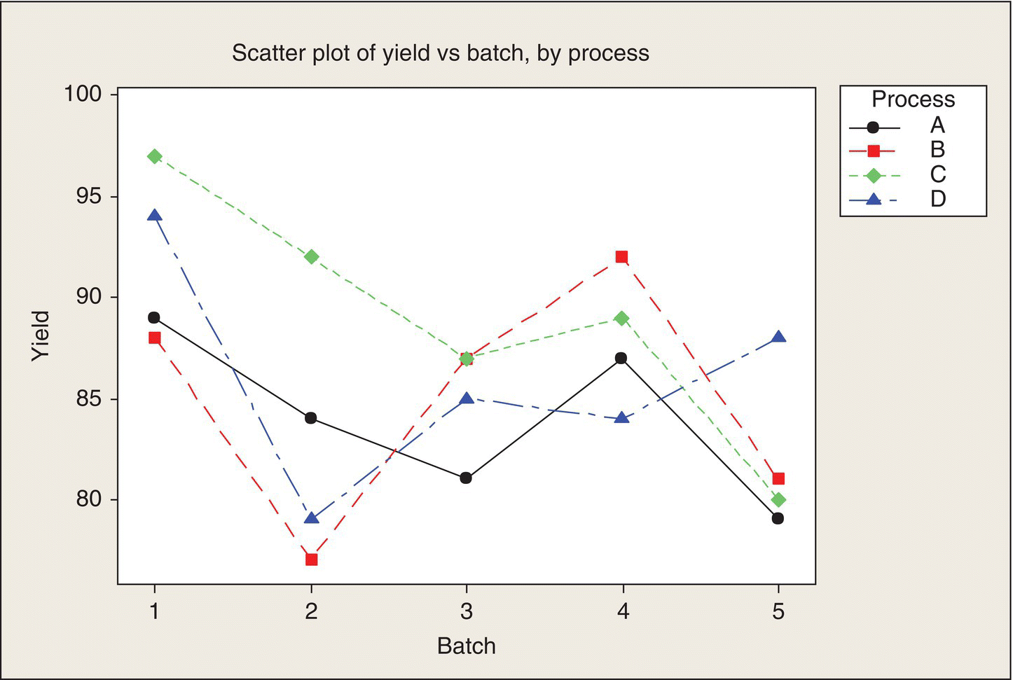
Figure 6.4 Data Plot for Penicillin Yield Experiment. .
Table 4.4, p. 146, BHH (2005), used with permission of John Wiley & Sons
Table 6.6 gives the ANOVA for these data. These results confirm what our eyeball analysis told us: there are no consistent differences among processes that stand out above the inherent variability of these processes (note the small F, large P). The marginally significant batch differences show that by blocking on batches, some reduction of experimental error was accomplished.
Table 6.6 Two-Way ANOVA: Yield versus Batch, Process.
| Source | DF | SS | MS | F | P |
| Batch | 4 | 264 | 66.0 | 3.50 | .04 |
| Process | 3 | 70 | 23.3 | 1.24 | .34 |
| Error | 12 | 226 | 18.8 | ||
| Total | 19 | 560 |
Where we might go from here depends on what is important. Because no real yield differences among processes were found, this means that the choice of process could be based on considerations other than yield. Cost, processing time, and environmental impact (say of process waste disposal) would be three such considerations.
Probably, the finding of most concern here is the finding of (what seems to me to be) substantial yield variability from batch to batch and among subbatches within a batch. This is akin to the finding in the first tomato fertilizer experience that there was a soil quality trend in the garden that contributed to tomato yield variability. In the next subsection, we will analyze these “components” of variability.
Components of variation
The finding that there was no evidence of real differences among processes means we can plot the data without showing the association of each data point with the process (treatment) it pertained to. Figure 6.5 shows the data by Batch. (Fig. 6.5 is Fig. 6.4 without linking the data points by process.)

Figure 6.5 Penicillin Yields by Batch.
The visual impression from Figure 6.5 is that the variability among the subbatch yields in each batch is consistent across batches and that the separation of the batches indicates that there is more variability among batches that one might expect from the amount of variability observed within batches. The impression is similar to that for the gear teeth data discussed in Chapter 4. This impression is quantified by carrying out a one-way ANOVA on the data: the only factor to consider is Batch. That ANOVA has the same structure as the ANOVA for a CRD with one Treatment factor. Table 6.7 gives the ANOVA.
Table 6.7 One-Way ANOVA: Penicillin Yield versus Batch.
| Source | DF | SS | MS | F | P |
| Batch | 4 | 264 | 66.0 | 3.34 | .04 |
| Error | 15 | 296 | 19.7 | ||
| Total | 19 | 560 |
The Error df and SS in this ANOVA are equal to the sum of the Process and Error df and SS in Table 6.4. The P-value for Batches is essentially the same as before.
(Note that I have done something that many texts never do: I have run two ANOVAs on the same data. Not arbitrarily, though. After the first ANOVA indicated one factor, process, was not a contributor to yields, I dropped that factor from consideration and did the appropriate resulting one-way ANOVA. In the same way, I transitioned from a plot that reflected both factors to a plot that just illustrated the more important factor—batch.)
Now, for the one-factor CRD, the follow-up analysis (Chapter 4) was to examine the treatment differences to identify the differences that stand out. That is not appropriate here. For example, we will never see Batches 1 and 3 again, so it makes no sense to ask whether the mean yields for Batches 1 and 3 are significantly different. Instead, our analysis is aimed at characterizing the two sources of variation in the data: (i) batch-to-batch variability and (ii) subbatch variability within batches. To provide a basis for this analysis, I will introduce a statistical model.
Let y ij denote the yield for batch i, subbatch j. A simple, additive statistical model for y ij (for yield data we might have gotten) is
where:
μ = overall average yield, b i = the (random) “effect” (on yield) of batch i; b i is assumed to have a Normal distribution with mean zero and standard deviation, σ b, e ij = (random) effect of subbatch i,j; e ij is assumed to have a Normal distribution with mean zero and standard deviation, σ e, which is constant across all batches, and b i and e ij are independent random variables.
This model is an example of what is called the “random effects model,” also a “variance components model,” on which there are extensive references in the statistical literature. In words, the model says that there is a random batch effect (modeled as a deviation from the overall average yield) that affects every subbatch in the batch and there is additional random variation among subbatches in a batch. The objective of the analysis is to estimate the two standard deviations in the model. Of course, we don’t observe μ or the batch and subbatch effects; all we observe is the subbatch yields. Nevertheless, ANOVA provides the quantities from which the two sigmas can be estimated.
First, the square root of the Error MS estimates σ
e, the standard deviation among subbatches in a batch. From Table 6.4, that estimate is ![]() . The df associated with this estimate is 15.
. The df associated with this estimate is 15.
Second, theory shows us that the Batch MS in the ANOVA estimates ![]() .(In more technical terms, the “expected value” of the Batch MS is equal to
.(In more technical terms, the “expected value” of the Batch MS is equal to ![]() . This means that if we repeatedly generated data according to the above variance component model and calculated the ANOVA table repeatedly, then the long-run average of the Batch MS would be this function of the two sigmas.) The factor of four is due to the fact that we had four subbatches in each batch. Note that if there was no batch-to-batch variability, σ
b would be equal to zero, so both the Error MS and the Batch MS would be estimating the same variance. That’s why the F-test is appropriate for detecting this additional source of variation. Because the Error MS estimates
. This means that if we repeatedly generated data according to the above variance component model and calculated the ANOVA table repeatedly, then the long-run average of the Batch MS would be this function of the two sigmas.) The factor of four is due to the fact that we had four subbatches in each batch. Note that if there was no batch-to-batch variability, σ
b would be equal to zero, so both the Error MS and the Batch MS would be estimating the same variance. That’s why the F-test is appropriate for detecting this additional source of variation. Because the Error MS estimates ![]() , we can estimate
, we can estimate ![]() by
by
For the penicillin yield data: estimated ![]() . (Note: The difference between BatchMS and ErrorMS can be negative, even though the quantity being estimated,
. (Note: The difference between BatchMS and ErrorMS can be negative, even though the quantity being estimated, ![]() , must be positive. Convention, in such a case, is to use zero as the estimated batch variance.)
, must be positive. Convention, in such a case, is to use zero as the estimated batch variance.)
The approximated df associated with this estimated variance is generally obtained by a method called Satterthwaite’s approximation (Wikipedia 2014b). Applying this method in this case results in the conclusion that the approximate df associated with this estimate is only two. This means that this is a very imprecise estimate. The 95% confidence interval on the underlying batch yield standard deviation is the interval: (1.8, 21%). With only five batches in the experiment, the maximum df we could have had for the estimate of batch variation is four. The within-batch variation, though, obscures what we can learn about batch-to-batch variation, so we only get 2 df worth of information, not 4 df. We need considerably more batches in the experiment to obtain a meaningful estimate of the batch standard deviation.
Sizing a Randomized Block Experiment
Consider an RBD with b blocks, k treatments, and r replicates of each treatment in each block (r > 1). The analysis of data from this design often comes down to the comparison of two treatment averages. The standard error of the difference between two treatment averages, say, treatments A and B, is

where EMS is the Error MS from the ANOVA, based on bt(r − 1) df. The denominator, br, reflects the fact that each average is an average of br observations; the factor of two reflects the fact that we are taking the difference between two independent averages.
This standard error is similar to that of a difference between two treatment means in an unpaired, two-treatment experiment with br experimental units in each treatment. The difference is that here the EMS is based on all the data, not just the data for the two treatment means being compared. Thus, if we use power curve criteria, plus a planning value for the error standard deviation, σ, for determining the number of observations in each treatment, as in Chapter 3, our analysis will be somewhat conservative because the actual error term will be based on more df than this two-sample analysis assumes. The n that results from that analysis can be equated to br, and the experiment planners can trade off the number of blocks, b, and the number of replicates, r.
In the case of an RBD with one replicate of each treatment in each block, the standard error of the difference between two treatment averages is

where now the EMS is based on (b − 1)(t − 1) degrees of freedom. A power curve-based analysis for a paired experiment could be used, somewhat conservatively, to determine the number of blocks required to satisfy specified power criteria.
True Replication
Example 5: Cookies
Let’s suppose we wanted to do an experiment to evaluate the effect of baking temperature on cookies made by three cookie-mix manufacturers. Here’s one way the experiment could be designed  :
:
- Prepare one batch of dough for each manufacturer: A, B, and C.
- Split each batch into three bowls of dough. Assign each bowl, randomly, to one of three temperatures selected for the experiment.
- Make four cookies from the dough in each bowl.
- Bake the four cookies simultaneously at their assigned temperature.
- Measure, by some means, the quality of each cookie.
This experiment looks a lot like the battery experiment; there are three manufacturers, three temperatures, and four cookies for each of the nine manufacturer–temperature combinations. A data table would look the same. But is it the same experimental design?
First, what is the experimental unit—the material to which the temperature treatment is independently applied? The answer is the eu is a group of four cookies formed from one bowl of dough. The response measured on the eu would be the average quality score of the four cookies that make up a single experimental unit.
Was the experiment a block design? Yes. A block is the three bowls of dough made from one batch of dough made with a single manufacturer’s mix. Thus, we have three blocks of three eus; each eu in a block is randomly assigned one of three temperatures. The design is an RBD with a single replicate of each treatment in each block.
What analyses can we do? We can do a two-way ANOVA, without replication. The F-test for temperature effects would have to use the block by temperature interaction as the denominator, which is valid under the assumption that the temperature effect is the same for all three manufacturers, that is, there is no block by treatment interaction. Presumably, though, a major reason for running the experiment is to find out, as in the battery experiment, if there is any difference in temperature sensitivity among the three mix manufacturers. This experiment makes it impossible to answer the question that motivated the experiment! I have seen this happen in real-world experiments with much more at stake than cookies.
Under the assumption of no block by temperature interaction, we can also do a test for block differences. However, because we created only one batch of dough for each manufacturer, we don’t know whether any apparent block differences are due to manufacturer or just reflect inherent batch-to-batch variability of batches independently prepared with the same mix. The experiment would need to have multiple batches from the same mix in order to separate manufacturer differences from batch variability.
If the ANOVA was done on the individual cookie scores and interpreted as though the design was an RBD with replication, the variability among the four cookies in the nine different mix-temperature combinations would be used to test for interaction as well as for temperature and mix effects. This assumed error term, though, is measuring the variability within an experimental unit and is therefore not appropriate for evaluating effects and interactions that are measured at the bowl-of-dough level. Because within-eu variability is apt to be smaller than among-eu variability, the tests may be unduly sensitive and lead to an unwarranted conclusion of real effects and interaction where none exist.
Bottom Line: Experimental design matters. You can’t tell a design by the layout of a spreadsheet—or a cookie sheet.
Example 6: Battery experiment revisited
In the battery experiment, the protocol was that individual batteries were stored at assigned temperatures and their lifetime was recorded. Suppose, though, that someone had noted that the temperature chamber and instrumentation would permit, say, all four batteries with a given plate material to be stored, attached to a load, and monitored simultaneously. That would save time. It would also sacrifice replication at the battery level. It makes this experiment equivalent to the (very flawed) cookie experiment. Now, the experimental unit is a group of four batteries with the same plate material. It’s the group of four that gets a single application of the temperature treatment. Individual batteries are samples from this experimental unit.
The natural response for the group (the eu) is the average lifetime of the four batteries in the group. This collapsing of the data results in an RBD with three blocks and three treatments and only single replicates in each block. Table 6.8 gives the ANOVA for these data.
Table 6.8 ANOVA for Modified Battery Experiment.
| Source | DF | SS | MS | F | P |
| Material | 2 | 2626 | 1313 | 2.24 | .22 |
| Temp | 2 | 9784 | 4895 | 8.34 | .04 |
| Error | 4 | 2348 | 587 | ||
| Total | 8 | 5953 |
(The first three lines of this ANOVA are the first three lines of the ANOVA in Table 6.3 divided by four. The factor of four is due to the fact that we are analyzing the means of four observations.) Had we done the experiment this way and gotten the same numerical results, we cannot tell from this ANOVA that there is significant interaction between materials and temperatures (we can’t test for it as we could when we processed the batteries singly and independently), and consequently, when we compare the differences among materials to our Error MS, based on the assumption of no block–treatment interaction, the conclusion is that there is no (statistically significant) difference in materials. That’s the wrong conclusion. What we know from the original experiment is that the different materials respond quite differently to increased temperature. This example should serve as a cautionary note about running single-replicate RBD. If resources permit, multiple-replicate RBD should be used.
Note: There is a way to test for a particular type of interaction in the case of only one replication in a two-way classification of data, such as a block–treatment cross-classification. This method is due to Tukey (1949), and it is illustrated in Box, Hunter, and Hunter (2005, p. 222) on data from the penicillin yield experiment.
Example 7: Boys’ shoes revisited
As discussed in the Introduction to this chapter, the boys’ shoes experiment in Chapter 3 was a randomized block experiment: there were 10 blocks (boys), each with two eus (feet), and two treatments (Materials A and B) assigned randomly in each block. Because each material could only be assigned to one foot, this is an RBD with no replication.
In Chapter 3, the boys’ shoes data were ultimately analyzed via the paired t-test. We obtained a t-value of 3.35, based on 9 df, and found the two-tailed P-value to be .009. Now that we’ve progressed to Chapter 6 and see that this experiment was a randomized block experiment, we can also address the question of a “real or random?” difference between the two sole materials by an ANOVA of the data. Table 6.9 gives this ANOVA.
Table 6.9 Two-Way ANOVA: Wear % versus Boy No., Material.
| Source | DF | SS | MS | F | P |
| Boy | 9 | 110.5 | 12.3 | 163.8 | .000 |
| Material | 1 | .84 | .84 | 11.2 | .009 |
| Error | 9 | .68 | .075 | ||
| Total | 19 | 112.00 |
The F-test statistic for comparing the materials is 11.2, based on 1 and 9 df (numerator and denominator), for which the P-value is, lo and behold, P = .009. In fact, the F-value is equal to the t-value squared (3.352 = 11.21, with a little difference due to round-off). Theory shows that an F-statistic based on (1, f) numerator and denominator df’s is equivalent to the square of a t-statistic based on f df. The difference, though, is the ANOVA doesn’t tell us the sign of the difference; the t-test does. Of course, the graphical displays one should or would do before either of these quantitative analyses would have told us the direction of the difference between materials: B had more wear than A.
As discussed, one purpose of blocking an experiment is to remove a source of variation from the comparison of treatments. The boys’ shoes experiment provides an example of the power of blocking. For the blocked experiment, the standard error of the average difference was SE(dbar) = .12%. This standard error was determined by dividing the standard deviation of the 10 differences by the square root of 10. That is exactly the same as the square root of the quantity: two times the Error MS in the Table 6.7 ANOVA divided by 10.
Now, suppose we had run a CRD in which we randomly assigned n boys to wear a pair of shoes of material A and another n boys to wear a material B pair. The standard error of the difference in this case (see the Chapter 3 discussion of the tomato fertilizer experiment) is ![]() , where s is the pooled boy-to-boy standard deviation within materials. The (boy-to-boy) standard deviations of both the A-data and the B-data are about 2.5%. Thus, for example, if the CRD experiment had been done with n = 10 boys in each material group, the standard error of the difference would have been
, where s is the pooled boy-to-boy standard deviation within materials. The (boy-to-boy) standard deviations of both the A-data and the B-data are about 2.5%. Thus, for example, if the CRD experiment had been done with n = 10 boys in each material group, the standard error of the difference would have been ![]() . This is approximately 10 times the SE(dbar) obtained from the blocked experiment. Because the SE is inversely proportional to the square root of n, this means it would have taken 102 or 100 times as many boys to get the same precision as the blocked experiment with 10 boys got. In other words, we would have to have had 1000 boys wearing A and 1000 boys wearing B to get the same precision as the blocked experiment got with 10 boys wearing one shoe of each material! Amazing. When the FLS who came up with the idea to block the experiment showed her boss this comparison, she was immediately promoted to Chief Statistical Officer and given a sizable bonus as well.
. This is approximately 10 times the SE(dbar) obtained from the blocked experiment. Because the SE is inversely proportional to the square root of n, this means it would have taken 102 or 100 times as many boys to get the same precision as the blocked experiment with 10 boys got. In other words, we would have to have had 1000 boys wearing A and 1000 boys wearing B to get the same precision as the blocked experiment got with 10 boys wearing one shoe of each material! Amazing. When the FLS who came up with the idea to block the experiment showed her boss this comparison, she was immediately promoted to Chief Statistical Officer and given a sizable bonus as well.
Nothing was said explicitly in Chapter 3 about the assumption of no block–treatment interaction. The issue was discussed, though, in other terms. In particular, we wondered whether the wear differences might depend on variables (such as age, weight, or activity levels of the boys in the experiment) that might have been useful in understanding the wear differences if they had been recorded. In the absence of such concomitant variables, we relied first on a randomization analysis and then a paired t-test and related confidence intervals, which treats the variation of differences as random variation, rather being due in part to variables such as boy’s weight, to evaluate the wear differences between B and A.
For the randomization analysis, the statistical model for data we might have gotten, under the assumption of no difference between A and B, was to randomly rearrange the A and B labels on the 10 pairs of wear data. The randomization test is validated simply by the act of randomly assigning treatments, so the no-interaction assumption does not come into play.
For the t-based analysis, the statistical model for data we might have gotten is a random sample of 10 differences from a single Normal distribution. The mean of that distribution, call it δ, is a constant. That is, the expected wear difference between B and A is the same for all boys. We didn’t have the data that would enable us to challenge that assumption. For example, suppose the underlying difference between sole wear of the two materials was related to a boy (block) characteristic such as number of hours the shoes were worn. Then, we would have single samples from ten different distributions, not 10 random samples from one distribution. This problem is the same as when in the first tomato fertilizer experiment it was found that yield depended on row position, thus contradicting the model of random samples from two Normal distributions. A key message you should take from this discussion is that randomization is the key to proper interpretation of experimental results, not ad hoc assumptions about Normal distributions.
Extensions of the RBD
Multifactor treatments and blocks—example: Penicillin experiment extended
The preceding examples in this chapter were all RBD experiments involving one blocking factor and one treatment factor. Just as in Chapter 5 we extended the CRD introduced in Chapter 4 to multifactor treatments, it is natural to extend the RBD to multifactor blocks, treatments, or both. This means that the experiment and subsequent statistical data analysis can address not just general differences among blocks or treatments but also the separate effects of block or treatment factors and the interaction among block factors, treatment factors, and between block and treatment factors.
Suppose you are the statistician who has been brought in to analyze the penicillin yield data and you ask the process engineers, “Tell me more about these four processes you want to compare. How are they defined; how are they different?” (Good consulting statisticians always ask lots of questions.) Eventually, you find out that two of the key processing variables are the time and temperature conditions under which fungi are fed nutrients. You further draw out the fact that the four processes of interest are defined by the four combinations of low and high temperature and short and long time. “Wow,” you say. “That’s a 2 × 2 factorial set of processes. We’ll be able to evaluate the separate effects of time and temperature and we’ll see whether time and temperature interact.” (More than once in real life I have found out that vague conditions, or processes, in an experiment were actually multifactor combinations of environmental or processing variables.) As a starting point in identifying the effects of the treatment factors, this treatment structure means that the ANOVA in Table 6.10 will have the following form.
Table 6.10 ANOVA for Penicillin Experiment, Extended.
| Source | DF | SS | MS | F | P |
| Batch | 4 | 264.0 | 66.0 | 3.50 | .04 |
| Process | 3 | 70.0 | 23.3 | 1.24 | .34 |
| Time | 1 | ||||
| Temp. | 1 | ||||
| Time × Temp. | 1 | ||||
| Error | 12 | 226.0 | 18.8 | ||
| Total | 19 | 560.0 |
(The entries for Time, Temp., and Time × Temp are indented to denote that these three lines in the ANOVA represent the decomposition of the three df for Process.)
If we could define the four processes in terms of time and temperature, we could separate the Process SS accordingly and find out what effects these two variables, singly and jointly—possible interaction—have on yield.)
Now, let’s look at the overall picture. The primary finding in the earlier variance component analysis (p. 191–194) is that there is appreciable batch-to-batch variation in yields but we need more data to get a better handle on this variation. We need to run more batches. Running more batches will also improve the sensitivity with which we can evaluate the process differences and the time and temperature effects. We might even consider obtaining multiple batches of corn steep liquor from multiple suppliers. Other suppliers might be more consistent than the one we are now using. Our analysis of these further experiments would address differences among suppliers with respect to average yield and with respect to the batch-to-batch variability of yield. The main thing we’ve learned about penicillin yield is that we need more data to understand it better. Such is the nature of science—and manufacturing.
Example 8: A blocks-only “experiment”—textile production
In Chapter 1, I defined an experiment as a controlled intervention in a process. In such an intervention, treatments are applied to experimental units and the resulting responses provide information about the treatment effects. There is a class of structured observation studies, though, in which multiple factors in, typically, a production process or a measurement process are studied with an aim of identifying dominant sources of variability in these processes. The findings of this study might be followed up with experiments aimed at finding processes changes that would reduce this variability. This is a fundamental method by which organizations can improve the quality of processes and products—reduced variability. For example, in the penicillin production example, the producer of corn steep liquor batches could look for ways to change the production process to produce more uniform (and high-yield) batches. In the bond-strength case study in Chapter 1, process engineers, aided by their FLS, found that the bonding and testing processes both were major sources of variability in the measured strength of bonds and subsequent experimentation and process changes led to reducing this variability. The following example, which deals with textile production, is from Scott and Triggs (2003).
In a textile factory, cloth is produced on a loom operated by one technician. Plant management (my story) is concerned about variation in the strength of the cloth produced in its factory. A study is undertaken in which cloth samples are produced by each of five technicians using each of seven looms. The two factors are thus crossed, and the five technicians and seven looms are randomly selected from large populations of each. (Visualize a large factory with at least dozens of looms and technicians.) Why the study was limited to five technicians and seven looms is not explained. I will speculate that it was to control the disruption of cloth production by the factory.
In the study, each technician produces one cloth sample on each loom so the result is 35 cloth samples (eus) cross-classified by loom and technician. No treatments, at this point, are applied to these 35 eus. Thus, we have 35 blocks, defined by the two blocking factors, loom and technician, with one eu in each block. The response measurement of interest is cloth strength, and Triggs’ random effects analysis leads to estimates of the loom and operator variance components. One might regard this as a uniformity study, similar in concept to the gauge studies discussed earlier.
Analysis 1: Plot the data
Figure 6.6 shows the data.

Figure 6.6 Cloth Strength by Technicians and Looms. Source: Scott and Triggs (2003, p. 91), used here by permission of Department of Statistics, University of Auckland.
First, note that the looms are arbitrarily numbered, so there is no horizontal trend to look for across looms. The fact that the lines are fairly flat for all five technicians indicates that the looms are fairly consistent. We see that machines are less variable than people because the main feature that stands out is the difference between technician 2 and her (I’ll assume, pardon the stereotype) peers. Her cloth samples had considerably higher strength than the other four technicians, by roughly 50%. (On second thought, maybe technician 2 is a guy, the other four are women, and, as we all know, men don’t read instructions.) What’s going on? Is one technician doing the right thing or are four? This pattern is not just a reflection of Normally distributed random variation, which one would assume in doing a variance components analysis of these data. Management needs to talk to these technicians to understand the causes of the variability among them and then take steps to reduce the variability.
Discussion
This example also reinforces the importance of plotting the data. One could feed these 35 cloth-strength measurements into statistical software and arrive at estimates of three variance components: loom to loom, technician to technician, and repeatability, which is the variation in repeated runs by the same technician on the same loom. Note that there was no replication in this experiment, so the repeatability variance component has to be estimated by the loom by technician interaction mean square in the ANOVA. The result of this analysis, as indicated by the data plot, is that the technician variance is the largest source of variation. This might/should lead the data analyst to look at the data and discover the patterns of variability noted earlier. We wouldn’t want to conclude from the quantitative results that, “Oh, people are variable, just random. Not much we can do about that.” This is not like the penicillin production example where we will never see the batches that were in the experiment again. These technicians and looms are still part of our production process, so we need to understand the causes of the differences we saw in the data. There may be cost implications of the study’s findings. Handled correctly, this study could lead management and labor to work together in a never-ending, data-driven, empowering, motivated quest for better quality, consistency, and cost-effectiveness!
Balanced Incomplete Block Designs
Example: Boys’ shoes revisited again
Suppose the head of shoe research comes to the statistician who had earned great respect with the paired experiment (randomized block) design to compare two shoe sole materials and says, “Now, we need to compare three different tread designs. How are you going to put three shoes on one boy? Huh, huh?”
Never fear. Statisticians have developed a class of designs called balanced incomplete block designs that can be used when the number of experimental units in a block is less than the number of treatments. In general, suppose there are b blocks available (or we can create them) with k experimental units in each and we want to evaluate t treatments (t > k). Catalogs exist (e.g., Cochran and Cox 1957, Chapter 11) that provide designs for feasible combinations of b, k, and t. For the requested shoe experiment, the appropriate incomplete block design would be as follows:
- Recruit n boys and randomly divide them into three groups (of the same size, if possible, though that’s not a requirement).
- In Group 1, randomly assign tread designs A and B to each boy’s two feet. In Group 2, randomly assign tread designs A and C to each boy’s two feet. In Group 3, randomly assign tread designs B and C to each boy’s two feet.
- Have the boys wear the shoes for some period of time and then measure appropriate characteristics of the soles, such as wear at key locations.
Thus, we run three paired designs. The analysis is a little tricky and beyond the scope of this text, but appropriate software can handle it. Just to indicate the issues, note that, say, the difference between designs A and B can be estimated from the Group 1 boys. Let dbar(A − B) denote the mean difference of the selected measurement for Group 1. This average difference estimates the A − B difference. Similarly, from Group 2 we get dbar(A − C) and from Group 3 we get dbar(B − C). Now, if we take the difference between the dbars for Groups 2 and 3, we get an estimate of the A − B difference based on the Groups 2 and 3 data. Thus, we have two estimates of the same difference: one from Group 1 and one from the difference between Groups 2 and 3. We need to combine them. The appropriate combination is a weighted average of the two A − B estimates.
Let’s suppose that the underlying variance from boy to boy of wear differences is the same for all three groups. Denote this common variance by σ 2. This assumption can be checked with the data. Suppose also that the number of boys in each group is the same for the three groups, say, r. Denote the two estimates of the A − B difference that the experiment provides as
The “hats” (carats) in these expressions indicate that we’re estimating the underlying average difference between A and B. The subscripts denote the Groups on which the estimates are based.
The variances of these two estimates are

Theory tells us that the optimum way to take a weighted average of two estimates of the same quantity is to weight the estimates inversely proportional to their variances. Thus, we weight (A − B)^1 by a weight of 2/3 and (A − B)^2,3 by 1/3 (the weights need to sum to 1.0). In terms of the average differences, this combined estimate of the underlying difference between tread designs A and B is

The variance of this estimate, by using the property that the variance of a linear combination of random variables is equal to the sum of the squares of the coefficients times the variance of each term, is equal to
Note that if we used only the Group 1 differences between A and B, the average difference would have a variance of σ 2/r. By including the other two Groups to get a combined estimate of the A − B difference, the denominator is increased by one-half. Thus, for example, if r = 10, the combined estimate is as precise as if we had run a paired experiment with only tread designs A and B with 15 boys. We have “borrowed information” about the A − B difference from Groups 2 and 3 and improved the precision with which the A − B difference can be estimated. In statistical literature, this information borrowing is called the recovery of interblock information. The 20 boys in Groups 2 and 3 in essence provide five boys worth of information about the A − B difference. This is yet another amazing accomplishment of good statistics.
This same sort of analysis can be carried out in general for incomplete block designs involving b blocks of k eus and t (>k) treatments.
Summary
This chapter has dealt primarily with the basic RBD: treatments are randomly assigned within blocks of experimental units. In addition to balanced incomplete block designs, statisticians have developed other designs that feature constraints on the definition of blocks and assignment of treatments. Examples of these designs are discussed in the next chapter.
Assignment
Choose a situation and issue(s) of interest to you. Design a randomized block experiment appropriate for investigating your issue or issues. Include at least one blocking factor and at least two treatment factors in your experiment:
- Define the experimental units, blocks, treatments, replication, and response measurement.
- Describe the protocol for applying treatments to experimental units and measuring the response.
- Describe how you would plot the resulting data.
- Lay out the ANOVA table for your experiment. Give the sources of variation and corresponding df.
- Discuss potential follow-on experiments.
References
- Box, G., Hunter, W. G., and Hunter, J. S. (1978, 2005) Statistics for Experimenters, John Wiley & Sons, Inc., New York.
- Cochran, W., and Cox, G. (1957) Experimental Designs, John Wiley & Sons, Inc., New York.
- Montgomery, D. (2001) Design and Analysis of Experiments, John Wiley & Sons, New York.
- Scott, A., and Triggs, C. (2003) Lecture Notes for Paper STATS 340, Department of Statistics, University of Auckland, Auckland.
- Tukey, J. (1949) One Degree of Freedom for Non-additivity, Biometrics, 5, 232–242.
- Wikipedia (2008) Penicillin, http://en.wikipedia.org/wiki/Penicillin#Mass_production.
- Wikipedia (2011) Arrhenius Equation, http://en.wikipedia.org/wiki/Arrhenius_equation.
- Wikipedia (2014a) Randomized Block Design, http://en.wikipedia.org/wiki/Randomized_block_design.
- Wikipedia (2014b) Welch–Satterthwaite Equation, http://en.wikipedia.org/wiki/Welch%E2%80%93Satterthwaite_equation.