Let's now look at how to extract the frequency spectrum from the spoken digits dataset. This dataset contains the recording of the digits spoken in the form of a .wav file. We will utilize the librosa library which is commonly used for audio data analysis. First, we need to install the package using the following command:
pip install librosa
For other methods of installing this library, you can look at https://github.com/librosa/librosa. We will use the MFCC, or Mel frequency cepstral coefficient feature, of the audio signal. MFCC is a kind of power spectrum that is obtained from short time frames of the signal. The main assumption is that for short durations of the order of 20 ms to 40 ms, the frequency spectrum does not change much. Therefore, the signal is sliced into these short time periods and the spectrum is computed for each slice. Fortunately, we do not have to worry about these details as the librosa library can do this for us. We utilize the following function to extract the MFCC feature:
def get_mfcc_features(fpath):
    raw_w,sampling_rate = librosa.load(fpath,mono=True)
    mfcc_features = librosa.feature.mfcc(raw_w,sampling_rate)
    if(mfcc_features.shape[1]>utterance_length):
        mfcc_features = mfcc_features[:,0:utterance_length]
    else:
        mfcc_features=np.pad(mfcc_features,((0,0),(0,utterance_length-mfcc_features.shape[1])),
                            mode='constant', constant_values=0)
    return mfcc_features
The librosa.load function loads the .wav file outputting the raw wav data raw_w and the sampling rate sampling_rate. The MFCC features are obtained by calling the librosa.feature.mfcc function on the raw data. Note that we also truncate the feature size to the utterance_length which is set to 35 in the code. This was set based on the average length of the utterance in the digit dataset. You can experiment with a higher value if required. For further details, you can take a look at the Jupyter Notebook under Chapter11/01_example.ipynb in this book's code repository. We will now print the shape of the feature and plot it to see what the power spectrum looks like:
import matplotlib.pyplot as plt
import librosa.display
%matplotlib inline
mfcc_features = get_mfcc_features('../../speech_dset/recordings/train/5_theo_45.wav')
plt.figure(figsize=(10, 6))
plt.subplot(2, 1, 1)
librosa.display.specshow(mfcc_features, x_axis='time')
print("Feature shape: ", mfcc_features.shape)
print("Features: ", mfcc_features[:,0])


Output:
Feature shape: (20, 35)
Features:[-5.16464322e+02 2.18720111e+02 -9.43628435e+01 1.63510496e+01
  2.09937445e+01 -4.38791200e+01 1.94267052e+01 -9.41531735e-02
 -2.99960992e+01 1.39727129e+01 6.60561909e-01 -1.14758965e+01
  3.13688180e+00 -1.34556070e+01 -1.43686686e+00 1.17119580e+01
 -1.54499037e+01 -1.13105764e+01 2.53027299e+00 -1.35725427e+01]
We can see that the spectrum (for spoken digit five here) consists of 20 features (the librosa default) for the 35 time slices of the audio signal. We can also see the MFCC feature values of the first time slice. We will now visualize the MFCC feature:

The regions toward the red (dark gray) color in the preceding figure indicates a large value of the MFCC coefficients while those toward the blue (light gray) indicates smaller values. Now, we will build a simple model for recognizing the digits in our audio data.